True colours and false colours images based on Sentinel-2 data on CopPhil
What is going to be covered?
The following example aims to present how to do basic visualizations using downloaded (API) or directly accessed (s3) data. It is divided into three main parts:
Visualization based on product (full) which was downloaded
Visualization based on product which was downloaded using Nodes() approach
Visualization based on product which was accessed using s3
Prerequisites
No. 1 Access to CopPhil site
You need a CopPhil hosting account, available at https://infra.copphil.philsa.gov.ph.
No. 2 Access to JupyterLab
JupyterLab used in this article is available here: https://jupyter.infra.copphil.philsa.gov.ph/hub/login?next=%2Fhub%2F.
No. 3 Working knowledge of JupyterLab
See article Introduction to JupyterLab on CopPhil
No. 4 Using API
This is an introductory example of obtaining EODATA using API calls, in Python:
Download satellite data using API on CopPhil
No. 5 Information on Sentinel-2 mission
Page Sentinel-2 mission shows basic information on Sentinel-2 mission, which is used in this article as a source of information.
What We Are Going To Cover
Preparing your environment
Visualizing based on product which was fully downloaded
Obtaining data
Creating a visualization (true color)
Visualizing based on product which was downloaded based on Nodes()
Obtaining data
Creating a visualization (true color)
Visualizing based on product which was downloaded using s3
Obtaining data
Creating a visualization (false color)
Summary
Prepare your environment
Upload necessary python libraries.
# HTTP requests
import requests

# JSON parser
import json

# data manipulation
import pandas as pd
import numpy as np

# image manipulation
import rasterio
import matplotlib.pyplot as plt
from rasterio.warp import calculate_default_transform, reproject, Resampling
from rasterio.transform import from_origin

# file manipulation
import os
import glob
import pathlib

# Interact with s3
import boto3
Visualize based on product which was fully downloaded
Obtain data
Follow Prerequisite No. 4 to obtain necessary data.
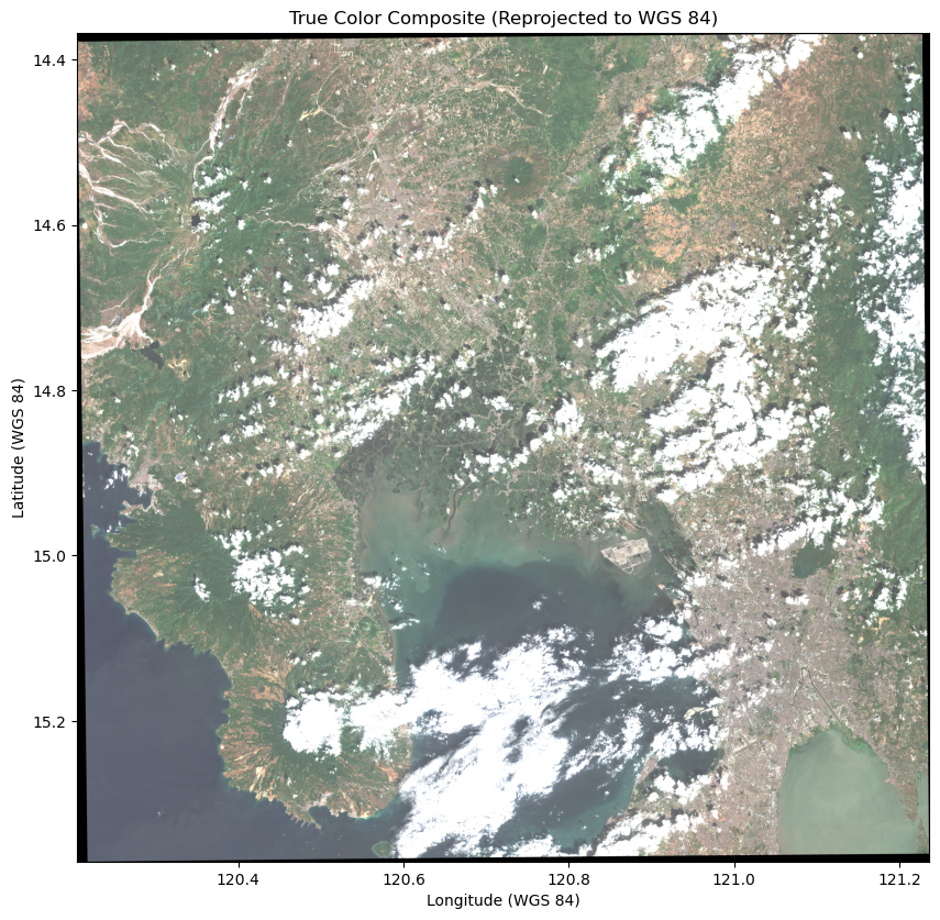
Create a visualization (true color)
- Define SAFE Folder Path
Specifies the path to the downloaded Sentinel-2 .SAFE folder for accessing satellite data.
- Set Up Band File Patterns
Defines search patterns for the Blue, Green, and Red band files (B2, B3, B4) in the IMG_DATA/R10m directory.
- Locate Band Files
Uses pathlib and rglob to find file paths matching the patterns, reads each band into a dictionary, and defaults to a zero array if a band is missing.
- Create True Color Composite
Stacks the bands (Red, Green, Blue) to create a true color image and normalizes values for visualization, scaling them to an 8-bit range (0–255).
- Extract CRS and Transformation
Reads the CRS (Coordinate Reference System) and transformation data from the Red band, which is required for reprojection.
- Define Target Projection (WGS 84)
Sets the target CRS to WGS 84 (EPSG:4326) and calculates the appropriate transformation and dimensions for reprojection.
- Reproject Composite Image
Reprojects each RGB band separately using bilinear resampling and stores them in a new array with the target CRS.
- Calculate Plot Extent
Computes the corner coordinates of the image for accurate geographic plotting.
- lot True Color Composite
Uses matplotlib to display the reprojected true color composite with longitude and latitude labeled on the WGS 84 coordinate system.
# Define the path to the downloaded SAFE folder
name_download = 'S2B_MSIL2A_20240211T021829_N0510_R003_T51PTS_20240211T050012.SAFE'  # Update this path
base_folder = f"{name_download}/{name_download}/GRANULE"

# Create a Path object
base_path = pathlib.Path(base_folder)

# Define patterns to search for the band files (updated for your directory structure)
band_patterns = {
    'B2': "*/IMG_DATA/R10m/*_B02_10m.jp2",  # Band 2 (Blue)
    'B3': "*/IMG_DATA/R10m/*_B03_10m.jp2",  # Band 3 (Green)
    'B4': "*/IMG_DATA/R10m/*_B04_10m.jp2"   # Band 4 (Red)
}

# Use rglob to find the actual file paths with wildcards and read the bands into a dictionary
bands = {}
for band_name, pattern in band_patterns.items():
    band_path = next(base_path.rglob(pattern), None)
    bands[band_name] = rasterio.open(band_path).read(1) if band_path else np.zeros((1, 1))

# Create the true color composite (R, G, B)
true_color = np.dstack((bands['B4'], bands['B3'], bands['B2']))  # Stack as (R, G, B)

# Normalize the data for visualization
true_color = np.clip(true_color, 0, 3000)
true_color = (true_color / 3000.0 * 255).astype(np.uint8)

# Get CRS and transformation from the red band
with rasterio.open(next(base_path.rglob(band_patterns['B4']))) as src:
    red_crs = src.crs
    red_transform = src.transform

# Reproject the true color composite to WGS 84 (EPSG:4326)
target_crs = 'EPSG:4326'
height, width = true_color.shape[:2]
bounds = rasterio.transform.array_bounds(height, width, red_transform)

# Calculate the transform and dimensions for the new projection
transform, width, height = calculate_default_transform(
    red_crs, target_crs, width, height, *bounds
)

# Prepare an empty array for the reprojected image
true_color_reprojected = np.empty((height, width, 3), dtype=np.uint8)

# Perform the reprojection for each band separately
for i in range(3):  # Loop over R, G, B
    reproject(
        true_color[:, :, i],  # The i-th band of the RGB composite
        true_color_reprojected[:, :, i],  # Destination
        src_transform=red_transform,  # Use red band transformation
        src_crs=red_crs,  # Source CRS
        dst_transform=transform,  # Destination transformation
        dst_crs=target_crs,  # Destination CRS
        resampling=Resampling.bilinear  # Bilinear resampling
    )

# Define corners for the extent of the plot
corners = np.array([[0, 0], [0, height], [width, height], [width, 0]])
x, y = rasterio.transform.xy(transform, corners[:, 1], corners[:, 0])

# Define the extent for the plot based on the transformed corners
ext = (x[0], x[2], y[0], y[1])

# Plot the reprojected true color composite using matplotlib
plt.figure(figsize=(10, 10))
plt.imshow(true_color_reprojected, extent=ext, origin='upper')
plt.title('True Color Composite')
plt.xlabel('Longitude (WGS 84)')
plt.ylabel('Latitude (WGS 84)')
plt.show()
Visualize based on product which was downloaded based on Nodes()
Obtain data
Follow the ‘Download satellite data using API on CopPhil’ article to obtain necessary data.
Create a visualization (true color)
- Define Folder Path
Sets base_folder to ‘tc_data’, where the Sentinel-2 band files are stored.
- Set Up Band File Patterns
Defines search patterns for Blue (B2), Green (B3), and Red (B4) bands based on typical Sentinel-2 naming conventions.
- Locate and Read Band Files
Uses pathlib and rglob to find each band file. Reads them into a dictionary or assigns a dummy zero array if a band file is missing.
- Create True Color Composite
Combines the bands (Red, Green, Blue) into a true color image. Clipping and scaling are applied to normalize pixel values within an 8-bit range (0–255) for visualization.
- Extract CRS and Transformation
Retrieves the Coordinate Reference System (CRS) and transformation matrix from the Red band for use in reprojection.
- Define Target Projection (WGS 84)
Sets the target projection to WGS 84 (EPSG:4326) and calculates the required transformation and new image dimensions.
- Reproject Composite Image
Reprojects each of the RGB bands individually using bilinear resampling, saving the transformed data to an array in the target CRS.
- Calculate Plot Extent
Computes the geographic coordinates of the image’s corners to set an accurate plot extent.
- Plot True Color Composite
Uses matplotlib to display the reprojected true color composite with labeled geographic coordinates (longitude and latitude) in WGS 84.
base_folder = 'tc_data'

# Create a Path object
base_path = pathlib.Path(base_folder)

# Define patterns to search for the band files (updated for your directory structure)
band_patterns = {
    'B2': "*_B02_10m.jp2",
    'B3': "*_B03_10m.jp2",
    'B4': "*_B04_10m.jp2"
}

# Use rglob to find the actual file paths with wildcards and read the bands into a dictionary
bands = {}
for band_name, pattern in band_patterns.items():
    band_path = next(base_path.rglob(pattern), None)
    bands[band_name] = rasterio.open(band_path).read(1) if band_path else np.zeros((1, 1))

# Create the true color composite (R, G, B)
true_color = np.dstack((bands['B4'], bands['B3'], bands['B2']))

# Normalize the data for visualization
true_color = np.clip(true_color, 0, 3000)
true_color = (true_color / 3000.0 * 255).astype(np.uint8)

# Get CRS and transformation from the red band
with rasterio.open(next(base_path.rglob(band_patterns['B4']))) as src:
    red_crs = src.crs  # Get CRS
    red_transform = src.transform

# Reproject the true color composite to WGS 84 (EPSG:4326)
target_crs = 'EPSG:4326'
height, width = true_color.shape[:2]
bounds = rasterio.transform.array_bounds(height, width, red_transform)

# Calculate the transform and dimensions for the new projection
transform, width, height = calculate_default_transform(
    red_crs, target_crs, width, height, *bounds
)

# Prepare an empty array for the reprojected image
true_color_reprojected = np.empty((height, width, 3), dtype=np.uint8)

# Perform the reprojection for each band separately
for i in range(3):  # Loop over R, G, B
    reproject(
        true_color[:, :, i],  # The i-th band of the RGB composite
        true_color_reprojected[:, :, i],  # Destination
        src_transform=red_transform,  # Use red band transformation
        src_crs=red_crs,  # Source CRS
        dst_transform=transform,  # Destination transformation
        dst_crs=target_crs,  # Destination CRS
        resampling=Resampling.bilinear  # Bilinear resampling
    )

# Define corners for the extent of the plot
corners = np.array([[0, 0], [0, height], [width, height], [width, 0]])
x, y = rasterio.transform.xy(transform, corners[:, 1], corners[:, 0])

# Define the extent for the plot based on the transformed corners
ext = (x[0], x[2], y[0], y[1])

# Plot the reprojected true color composite using matplotlib
plt.figure(figsize=(10, 10))
plt.imshow(true_color_reprojected, extent=ext, origin='upper')
plt.title('True Color Composite')
plt.xlabel('Longitude (WGS 84)')
plt.ylabel('Latitude (WGS 84)')
plt.show()

Visualize based on product which was downloaded using s3
Obtain data
Follow the ‘Download satellite data using s3 on CopPhil’ article to obtain necessary data.
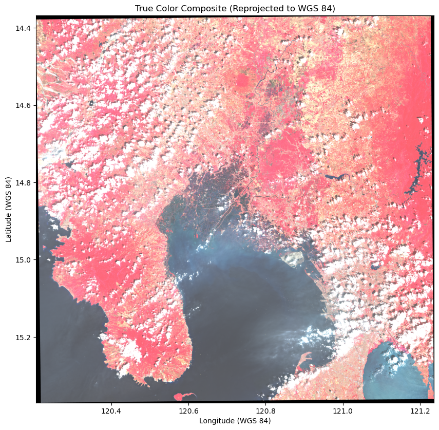
Create a visualization (false color)
- Define SAFE Folder Path
Specifies the path to the Sentinel-2 .SAFE folder, pointing to where the satellite data is stored (on s3).
- Set Up Band File Patterns
Defines search patterns for the bands needed to create the true color image: Near Infrared (B8), Red (B4), and Green (B2).
- Locate and Read Band Files
Uses pathlib and rglob to find each band file, reads them into a dictionary, and defaults to a zero array if a band is not found.
- Create False Color Composite
Combines the bands in an RGB order (Red, Green, Blue) using np.dstack to create a true color composite image. Data values are clipped and scaled to an 8-bit - display range (0–255).
- Extract CRS and Transformation
Retrieves the Coordinate Reference System (CRS) and transformation matrix from the Green band for accurate reprojection.
- Define Target Projection (WGS 84)
Sets the target CRS to WGS 84 (EPSG:4326) and calculates the required transformation and new dimensions for the reprojected image.
- Reproject Composite Image
Reprojects each band separately using bilinear resampling and stores the transformed data in a new array with the target CRS.
- Calculate Plot Extent
Computes the geographic corner coordinates of the image to set the extent for the plot.
- Plot False Color Composite
Uses matplotlib to display the reprojected true color image with geographic labels for longitude and latitude in the WGS 84 system.
# Define the path to the downloaded SAFE folder
name_download = '/eodata/Sentinel-2/MSI/L2A/2024/03/07/S2A_MSIL2A_20240307T021541_N0510_R003_T51PTS_20240307T053851.SAFE'  # Update this path
base_folder = f"{name_download}/GRANULE"

# Create a Path object
base_path = pathlib.Path(base_folder)

# Define patterns to search for the band files
band_patterns = {
    'B3': "*/IMG_DATA/R10m/*_B03_10m.jp2",
    'B4': "*/IMG_DATA/R10m/*_B04_10m.jp2",
    'B8': "*/IMG_DATA/R10m/*_B08_10m.jp2"
}

# Use rglob to find the actual file paths with wildcards and read the bands into a dictionary
bands = {}
for band_name, pattern in band_patterns.items():
    band_path = next(base_path.rglob(pattern), None)
    bands[band_name] = rasterio.open(band_path).read(1) if band_path else np.zeros((1, 1))

# Create the true false composite (NIR, R, G)
true_color = np.dstack((
    bands.get('B8', np.zeros((1, 1))),
    bands.get('B4', np.zeros((1, 1))),
    bands.get('B3', np.zeros((1, 1)))
))

# Normalize the data for visualization
true_color = np.clip(true_color, 0, 3000)
true_color = (true_color / 3000.0 * 255).astype(np.uint8)


# Get CRS and transformation from the red band
with rasterio.open(next(base_path.rglob(band_patterns['B4']))) as src:
    red_crs = src.crs
    red_transform = src.transform

# Reproject the true color composite to WGS 84 (EPSG:4326)
target_crs = 'EPSG:4326'
height, width = true_color.shape[:2]
bounds = rasterio.transform.array_bounds(height, width, red_transform)

# Calculate the transform and dimensions for the new projection
transform, width, height = calculate_default_transform(
    red_crs, target_crs, width, height, *bounds
)

# Prepare an empty array for the reprojected image
true_color_reprojected = np.empty((height, width, 3), dtype=np.uint8)

# Perform the reprojection for each band separately
for i in range(3):  # Loop over NIR, R, G
    reproject(
        true_color[:, :, i],  # The i-th band of the RGB composite
        true_color_reprojected[:, :, i],  # Destination
        src_transform=red_transform,  # Use red band transformation
        src_crs=red_crs,  # Source CRS
        dst_transform=transform,  # Destination transformation
        dst_crs=target_crs,  # Destination CRS
        resampling=Resampling.bilinear  # Bilinear resampling
    )

# Define corners for the extent of the plot
corners = np.array([[0, 0], [0, height], [width, height], [width, 0]])
x, y = rasterio.transform.xy(transform, corners[:, 1], corners[:, 0])

# Define the extent for the plot based on the transformed corners
ext = (x[0], x[2], y[0], y[1])

# Plot the reprojected true color composite using matplotlib
plt.figure(figsize=(10, 10))
plt.imshow(true_color_reprojected, extent=ext, origin='upper')
plt.title('False Color Composite')
plt.xlabel('Longitude (WGS 84)')
plt.ylabel('Latitude (WGS 84)')
plt.show()
Summary
This notebook processes Sentinel-2 data to create a true color and false color composites from selected bands. It reprojects the image to the WGS 84 coordinate system and visualizes it with geographic coordinates (longitude and latitude).