Agriculture and food security monitoring using Sentinel-2 data in JupyterLab on CopPhil

The following example aims to present how to interact with the catalogue, download EO data products and do some basic visualization.

• Search for Sentinel-2 L2A products using specific filters

• Download data

• Calculate Normalized Difference Vegetation Index (NDVI)

• Visualize Normalized Difference Vegetation Index over the image

• Visualize Normalized Difference Vegetation Index over the specific field

• Calculate and visualize other indices: Normalized Difference Infrared Index (NDII) and Normalized Difference Red-Edge (NDRE)

Prerequisites

No. 1 Access to CopPhil site

You need a CopPhil hosting account, available at https://infra.copphil.philsa.gov.ph.

No. 2 Access to JupyterLab

JupyterLab used in this article is available here: https://jupyter.infra.copphil.philsa.gov.ph/hub/login?next=%2Fhub%2F.

No. 3 Working knowledge of JupyterLab

See article Introduction to JupyterLab on CopPhil

No. 4 Using API

This is an introductory example of obtaining EODATA using API calls, in Python:

Download satellite data using API on CopPhil

No. 5 Information on Sentinel-2 mission

Page Sentinel-2 mission shows basic information on Sentinel-2 mission, which is used in this article as a source of information.

No. 6 Use Geo science kernel

Geo science kernel has preinstalled all of the Python libraries in this article:

Python 3 kernel and Geo science kernel in JupyterLab on CopPhil

What We Are Going To Do

• Prepare your environment

• Search for Sentinel-2 L2A products

  • Build a query

  • Inspect results of the request

• Download data

• Authentication

• Select product to be downloaded

• Unpack data

• Visualize data

  • Define a function which aims to load a bands of the Sentinel-2 image, including metadata

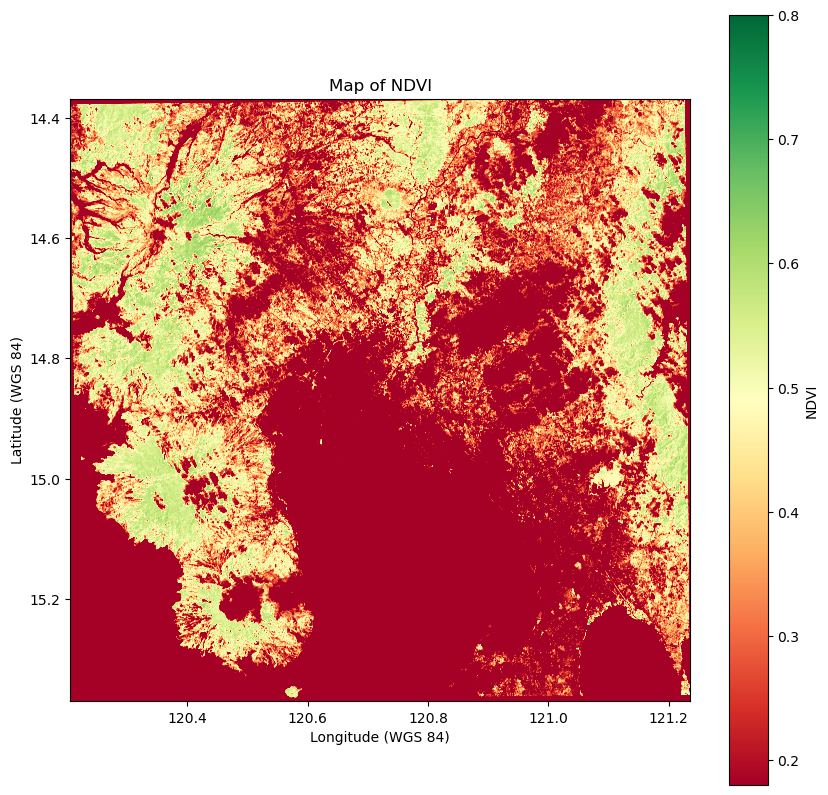
  • Create a map of NDVI over the area covered by the image

  • NDVI - Normalized Difference Vegetation Index

  • Calculate NDVI

• Visualization

  • Map of selected area

  • Create a map of NDII over the area covered by the image

  • NDII - Normalized Difference Infrared Index

  • Calculate NDII

  • Create a map of NDRE over the area covered by the image

  • NDRE - Normalized Difference Red Edge

  • Calculate NDRE

• Summary

Prepare your environment

Upload necessary python libraries.

# HTTP requests
import requests

# JSON parser
import json


# data manipulation
import pandas as pd
import numpy as np

# image manipulation
import rasterio
from rasterio.warp import calculate_default_transform, reproject, Resampling
import matplotlib.pyplot as plt
import matplotlib.ticker as ticker
import numpy as np

# file manipulation
import pathlib
import zipfile
import os

Search for Sentinel-2 L2A products

Let’s start with obtaining some data. This part is also covered by Download satellite data using API on CopPhil.

Build a query

In order to find desired products it is needed to determinate some specific filters:

collection_name

Sentinel-2

product_type

MSIL2A

aoi

extent (coordinates) of the area of interest (WGS84)

search_period_start

time range - start date

search_period_end

time range - end date

max_cloud_cover

maximum cloud cover (%) fo the image

# base URL of the product catalogue
catalogue_odata_url = "https://catalogue.infra.copphil.philsa.gov.ph/odata/v1"

# search parameters
collection_name = "SENTINEL-2"
product_type = "S2MSI2A"
aoi = "POLYGON((120.962986 14.598416, 120.995964 14.599182, 120.999658 14.563436, 120.960348 14.567522, 120.962986 14.598416))"
search_period_start = "2024-01-01T00:00:00.000Z"
search_period_end = "2024-09-30T00:00:00.000Z"

search_query = f"{catalogue_odata_url}/Products?$filter=Collection/Name eq '{collection_name}' and Attributes/OData.CSC.StringAttribute/any(att:att/Name eq 'productType' and att/OData.CSC.StringAttribute/Value eq '{product_type}') and OData.CSC.Intersects(area=geography'SRID=4326;{aoi}') and ContentDate/Start gt {search_period_start} and ContentDate/Start lt {search_period_end}"

max_cloud_cover = 20

search_query_cloud = f"{search_query} and Attributes/OData.CSC.DoubleAttribute/any(att:att/Name eq 'cloudCover' and att/OData.CSC.DoubleAttribute/Value le {max_cloud_cover})"
print(f"""\n{search_query.replace(' ', "%20")}\n""")

https://catalogue.infra.copphil.philsa.gov.ph/odata/v1/Products?$filter=Collection/Name%20eq%20'SENTINEL-2'%20and%20Attributes/OData.CSC.StringAttribute/any(att:att/Name%20eq%20'productType'%20and%20att/OData.CSC.StringAttribute/Value%20eq%20'S2MSI2A')%20and%20OData.CSC.Intersects(area=geography'SRID=4326;POLYGON((120.962986%2014.598416,%20120.995964%2014.599182,%20120.999658%2014.563436,%20120.960348%2014.567522,%20120.962986%2014.598416))')%20and%20ContentDate/Start%20gt%202024-01-01T00:00:00.000Z%20and%20ContentDate/Start%20lt%202024-09-30T00:00:00.000Z

Inspect results of the request

Show the number of found products which fits into filters requirements and get a list of names and id’s of images which fits the query.

response = requests.get(search_query_cloud).json()
result = pd.DataFrame.from_dict(response["value"])

id_list = []
for element in response['value']:
    id_value = element['Id']
    id_list.append(id_value)

for id in id_list:
    print(id)

name_list = []
for element in response['value']:
    name_value = element['Name']
    name_list.append(name_value)

for name in name_list:
    print(name)

print(f'Number of products which meets query filters: {len(result)}')

51b58ff8-4fd5-4fe3-b2f0-beebfee95bab
f5c26c11-d72d-4c91-80ec-fd7428c0d518
dfe46249-bc17-401f-bf9a-bcc05efe77c7
cbdd1d86-52ac-4ee7-aa33-306019d525db
af473459-5577-48ba-a852-2607f7fe8357
4acc616f-1f77-460b-867e-4d3452dee225
S2B_MSIL2A_20240211T021829_N0510_R003_T51PTS_20240211T050012.SAFE
S2A_MSIL2A_20240307T021541_N0510_R003_T51PTS_20240307T053851.SAFE
S2B_MSIL2A_20240302T021609_N0510_R003_T51PTS_20240302T043128.SAFE
S2B_MSIL2A_20240421T021529_N0510_R003_T51PTS_20240421T043611.SAFE
S2A_MSIL2A_20240416T021611_N0510_R003_T51PTS_20240416T075854.SAFE
S2A_MSIL2A_20240426T021611_N0510_R003_T51PTS_20240426T075954.SAFE
Number of products which meets query filters: 6

Get a name and id of the first image which fits the query and an info when the image was generated.

id_download = response['value'][0]['Id']
name_download = response['value'][0]['Name']
print(f'id: {id_download}, name {name_download}')

image_date = response['value'][0]['ContentDate']['Start']
print(f'Image was generated on {image_date}')

id: 51b58ff8-4fd5-4fe3-b2f0-beebfee95bab, name S2B_MSIL2A_20240211T021829_N0510_R003_T51PTS_20240211T050012.SAFE
Image was generated on 2024-02-11T02:18:29.024000Z

Then, we are going to work with data which was acquired on 2024-02-11.

Download data

Authentication

Log in to the portal. If status_code=200, it means you are logged successfully.

# Provide CopPhil account credentials - replace with your own data

username = 'username'
password = 'user's password'

auth_server_url = "https://auth.copphil.cloudferro.com/auth/realms/copphilinfra/protocol/openid-connect/token"
data = {
    "client_id": "copphil-public",
    "grant_type": "password",
    "username": username,
    "password": password,
}

response = requests.post(auth_server_url, data=data, verify=True, allow_redirects=False)
access_token = json.loads(response.text)["access_token"]
status_code = response.status_code
print(status_code)

200

Select product to be downloaded

From the list which was provided in the previous stage and based on image name and id, download the proper image.

url_download = f'https://download.infra.copphil.philsa.gov.ph/odata/v1/Products({id_download})/$value'
url_download_using_token = url_download + '?token=' + access_token

# downloads the file
pulling = requests.get(url_download_using_token)
open(f"{name_download}.zip", 'wb').write(pulling.content)

1156520968

Unpack data

Unzip downloaded folder.

# Unzipping the file
with zipfile.ZipFile(f'{name_download}.zip', 'r') as zip_ref:
    zip_ref.extractall(f'{name_download}')

# Check if unzipped successfully
if os.path.exists(f'{name_download}'):
    print(f"Unzipped successfully into {name_download}")
else:
    print("Unzipping failed.")

Unzipped successfully into S2B_MSIL2A_20240211T021829_N0510_R003_T51PTS_20240211T050012.SAFE

Visualize data

In this section, there will be presented how calculate vegetation indices (NDVI, NDII and NDRE) and how to prepare a maps of these indices.

Vegetation indices are useful for monitoring agriculture because they allow for real-time assessment of plant health and condition. They enable precise tracking of vegetation changes, which helps optimize irrigation and fertilization.

Define a function which aims to load a bands of the Sentinel-2 image, including metadata

Firstly, define a function which aims to load necessary data into environment.

• Load a band

• Get CRS (coordinate system’s EPSG)

• Get the affine transformation

def load_band(band_path):
    with rasterio.open(band_path) as src:
        band = src.read(1)                  # Read the first band
        crs = src.crs                       # Get the CRS of the image
        transform = src.transform           # Get the affine transformation
    return band, crs, transform

Create a map of NDVI over the area covered by the image

NDVI - Normalized Difference Vegetation Index

The Normalized Difference Vegetation Index (NDVI) is a widely used remote sensing index to assess vegetation health, density, and productivity. It measures the difference between near-infrared (NIR) light, which vegetation strongly reflects, and red light, which plants absorb.

Applications of NDVI:

Agriculture

Farmers use NDVI to monitor crop health and detect areas that need attention (irrigation, fertilization).

Forestry

Foresters monitor forest health and detect deforestation.

Environmental Monitoring

NDVI helps detect ecosystem changes, track desertification, or monitor recovery from natural disasters.

\[NDVI = \frac{{\text{NIR} - \text{Red}}}{{\text{NIR} + \text{Red}}}\]

Red

Red band (Sentinel-2 - B04)

NIR

Near-infrared band (Sentinel-2 - B08/B8A)

NDVI Value	Interpretation
+1	Dense, healthy vegetation
0.6 to 0.9	High vegetation, forest, or dense green crops
0.2 to 0.5	Sparse or moderate vegetation (grasslands, shrubs)
0.0 to 0.2	Bare soil, rocks, or very sparse vegetation
0 to -1	Non-vegetated surfaces (water, snow, urban areas)

Calculate NDVI

• The script defines paths to Red and Near-Infrared (NIR) bands within a Sentinel-2 .SAFE folder, using wildcards to locate files accurately.

• It loads these bands along with their Coordinate Reference System (CRS) and transformation details for geospatial alignment.

• NDVI is calculated by dividing the difference between NIR and Red bands by their sum, with a small constant added to avoid division by zero errors.

# Define paths to bands (inside your .SAFE folder)
base_folder = f"{name_download}/{name_download}/GRANULE"
band_red_pattern = "*/IMG_DATA/R10m/*_B04_10m.jp2"
band_nir_pattern = "*/IMG_DATA/R10m/*_B08_10m.jp2"

# Create a Path object
base_path = pathlib.Path(base_folder)

# Use rglob to find the actual file paths with wildcards
band_red_path = next(base_path.rglob(band_red_pattern), None)
band_nir_path = next(base_path.rglob(band_nir_pattern), None)

# Load the Red and NIR bands with their CRS and transformation
red, red_crs, red_transform = load_band(band_red_path)
nir, nir_crs, nir_transform = load_band(band_nir_path)

# Calculate NDVI
ndvi = (nir.astype(float) - red.astype(float)) / (nir + red + 1e-10)

Visualization

• Reproject to WGS 84 from native image CRS

• Create a map

# Reproject NDVI to WGS 84 (EPSG:4326)
target_crs = 'EPSG:4326'
height, width = red.shape
bounds = rasterio.transform.array_bounds(height, width, red_transform)

# Calculate the transform and dimensions for the new projection
transform, width, height = calculate_default_transform(
    red_crs, target_crs, width, height, *bounds
)

# Prepare the NDVI array to be reprojected with the new shape
ndvi_reprojected = np.empty((height, width), dtype=np.float32)

# Perform the reprojection into the new array
reproject(
    ndvi,
    ndvi_reprojected,
    src_transform=red_transform,
    src_crs=red_crs,
    dst_transform=transform,
    dst_crs=target_crs,
    resampling=Resampling.bilinear
)

corners = np.array([[0, 0], [0, height], [width, height], [width, 0]])

# Transform pixel coordinates to geographic coordinates
x, y = rasterio.transform.xy(transform, corners[:, 1], corners[:, 0])

# Define the extent for the plot based on the transformed corners
ext = (x[0], x[2], y[0], y[1])


# Plot the reprojected NDVI
plt.figure(figsize=(10, 10))
plt.imshow(ndvi_reprojected, cmap='RdYlGn', extent=ext, origin='upper', vmin=0.8, vmax=0.2)
plt.colorbar(label='NDVI')
plt.title("Map of NDVI")
plt.xlabel('Longitude (WGS 84)')
plt.ylabel('Latitude (WGS 84)')
plt.show()

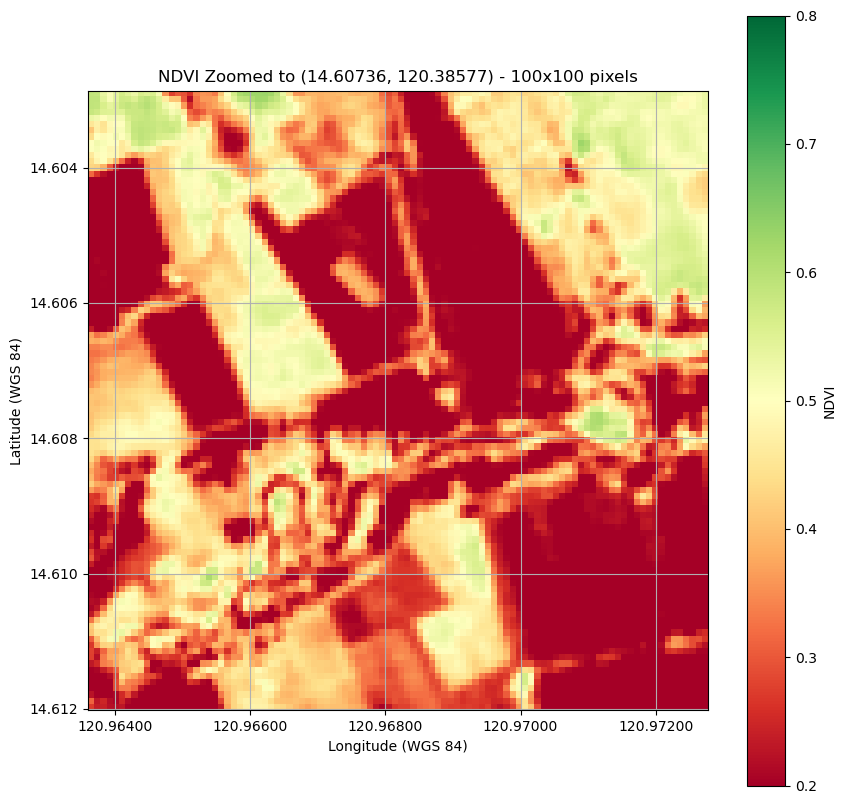
Map of selected area

• Limit display to selected area (100x100 pixels around 14.60736 N, 120.38577 E)

• Create a map

Define a function which convert latitude and longitude to pixel coordinates

# Convert latitude and longitude to pixel coordinates
def latlon_to_pixel(transform, lat, lon):
    x, y = lon, lat
    pixel_row, pixel_col = ~transform * (x, y)
    return int(pixel_row), int(pixel_col)

Clip image to the selected area and calculate NDVI.

# Define the coordinates to zoom into
latitude = 14.60736
longitude = 120.38577

# Get pixel coordinates for the target latitude and longitude
pixel_row, pixel_col = latlon_to_pixel(transform, latitude, longitude)

# Define the size of the zoom window (100x100 pixels around the point)
window_size = 100
row_start = max(0, pixel_row - window_size // 2)
row_end = min(height, pixel_row + window_size // 2)
col_start = max(0, pixel_col - window_size // 2)
col_end = min(width, pixel_col + window_size // 2)

# Crop the NDVI image to this window
ndvi_zoomed = ndvi_reprojected[row_start:row_end, col_start:col_end]

# Clip NDVI values to [-1, 1] for better visualization
ndvi_zoomed = np.clip(ndvi_zoomed, -1, 1)

# Calculate the new geographic bounds for the zoomed area
new_xmin = transform[2] + transform[0] * col_start + transform[1] * row_start  # Longitude min
new_xmax = transform[2] + transform[0] * col_end + transform[1] * row_start    # Longitude max
new_ymin = transform[5] + transform[4] * col_start + transform[3] * row_start  # Latitude min
new_ymax = transform[5] + transform[4] * col_end + transform[3] * row_end      # Latitude max
new_bounds = (new_xmin, new_xmax, new_ymin, new_ymax)

Plot a clipped image.

plt.figure(figsize=(10, 10))

# Debugging: Print out the shape of the zoomed NDVI image
print(f"Zoomed NDVI shape: {ndvi_zoomed.shape}")

plt.imshow(ndvi_zoomed, cmap='RdYlGn',
           extent=new_bounds,
           origin='upper', vmin=0.2, vmax=0.8)  # Set vmin and vmax for color scaling

# Set axis limits to match the geographic extents
plt.xlim(new_bounds[0], new_bounds[1])  # Longitude limits
plt.ylim(new_bounds[2], new_bounds[3])  # Latitude limits

# Format the longitude axis to prevent scientific notation
plt.gca().xaxis.set_major_formatter(ticker.FuncFormatter(lambda x, _: f"{x:.5f}"))

# Add grid and colorbar for better visualization
plt.colorbar(label='NDVI')
plt.title(f"NDVI Zoomed to ({latitude}, {longitude}) - 100x100 pixels")
plt.xlabel('Longitude (WGS 84)')
plt.ylabel('Latitude (WGS 84)')
plt.grid(True)

# Show the plot
plt.show()

Zoomed NDVI shape: (100, 100)

Create a map of NDII over the area covered by the image

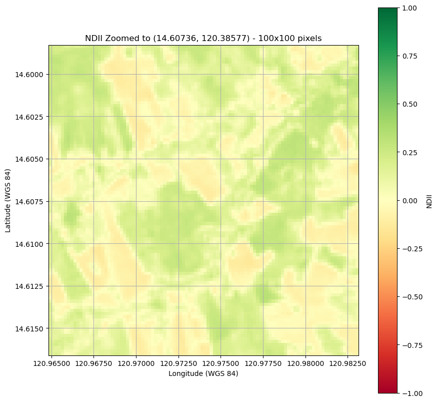
NDII - Normalized Difference Infrared Index

The Normalized Difference Infrared Index (NDII) is a remote sensing index used to assess the moisture content of vegetation. It is particularly sensitive to water in plant canopies and is often used to monitor drought conditions, forest health, and the moisture status of crops.

Applications of NDII:

Drought Monitoring

Identifies areas of vegetation under drought stress by detecting moisture levels.

Agriculture

Monitors the water status of crops, helping optimize irrigation strategies.

Forestry

Assesses the health of forests and their susceptibility to wildfires by evaluating canopy moisture.

Environmental Monitoring

Detects large-scale changes in ecosystems caused by moisture variability.

Precision Agriculture

Helps farmers manage fertilization and irrigation by detecting nutrient deficiencies and water stress early.

\[NDII = \frac{{\text{NIR} - \text{SWIR}}}{{\text{NIR} + \text{SWIR}}}\]

NIR

Near-infrared band (Sentinel-2 - B08/B8A)

SWIR

Shortwave infrared (Sentinel-2 - B11)

NDII Value	Interpretation
+1	High moisture content in vegetation
0.2 to 0.9	Healthy vegetation with adequate moisture
0.0 to 0.2	Moderate moisture levels; vegetation may be under stress
-0.2 to 0.0	Low moisture content; vegetation likely stressed
Below -0.2	Very low or no moisture; drought stress or bare soil

Calculate NDII

• The script defines paths to Short Infrared (SWIR) and Near-Infrared (NIR) bands within a Sentinel-2 .SAFE folder, using wildcards to locate files accurately.

• It loads these bands along with their Coordinate Reference System (CRS) and transformation details for geospatial alignment.

• NDII is calculated by dividing the difference between NIR and Red bands by their sum, with a small constant added to avoid division by zero errors.

# Define paths to bands (inside your .SAFE folder)
base_folder = f"{name_download}/{name_download}/GRANULE"
band_nir_pattern = "*/IMG_DATA/R20m/*_B8A_20m.jp2"
band_swir_pattern = "*/IMG_DATA/R20m/*_B11_20m.jp2"

# Create a Path object
base_path = pathlib.Path(base_folder)

# Use rglob to find the actual file paths with wildcards
band_nir_path = next(base_path.rglob(band_nir_pattern), None)
band_swir_path = next(base_path.rglob(band_swir_pattern), None)

# Load the Red and NIR bands with their CRS and transformation
nir, nir_crs, red_transform = load_band(band_nir_path)
swir, swir_crs, nir_transform = load_band(band_swir_path)

# Calculate NDII
ndii = (nir.astype(float) - swir.astype(float)) / (nir + swir + 1e-10)

Reproject to WGS 84.

# Reproject NDII to WGS 84 (EPSG:4326)
target_crs = 'EPSG:4326'
height, width = red.shape
bounds = rasterio.transform.array_bounds(height, width, red_transform)

# Calculate the transform and dimensions for the new projection
transform, width, height = calculate_default_transform(
    red_crs, target_crs, width, height, *bounds
)

# Prepare the NDVI array to be reprojected with the new shape
ndii_reprojected = np.empty((height, width), dtype=np.float32)

# Perform the reprojection into the new array
reproject(
    ndii,
    ndii_reprojected,
    src_transform=red_transform,
    src_crs=red_crs,
    dst_transform=transform,
    dst_crs=target_crs,
    resampling=Resampling.bilinear
)

(array([[0., 0., 0., ..., 0., 0., 0.],
        [0., 0., 0., ..., 0., 0., 0.],
        [0., 0., 0., ..., 0., 0., 0.],
        ...,
        [0., 0., 0., ..., 0., 0., 0.],
        [0., 0., 0., ..., 0., 0., 0.],
        [0., 0., 0., ..., 0., 0., 0.]], dtype=float32),
 Affine(0.00018313590139129615, 0.0, 120.20554290877753,
        0.0, -0.00018313590139129615, 15.375878870057374))

Clip image to the selected area

# Define the coordinates to zoom into
latitude = 14.60736
longitude = 120.38577

# Get pixel coordinates for the target latitude and longitude
pixel_row, pixel_col = latlon_to_pixel(transform, latitude, longitude)

# Define the size of the zoom window (100x100 pixels around the point)
window_size = 100
row_start = max(0, pixel_row - window_size // 2)
row_end = min(height, pixel_row + window_size // 2)
col_start = max(0, pixel_col - window_size // 2)
col_end = min(width, pixel_col + window_size // 2)

# Crop the NDII image to this window
ndii_zoomed = ndii_reprojected[row_start:row_end, col_start:col_end]

# Clip NDII values to [-1, 1] for better visualization
ndii_zoomed = np.clip(ndii_zoomed, -1, 1)

# Calculate the new geographic bounds for the zoomed area
new_xmin = transform[2] + transform[0] * col_start + transform[1] * row_start  # Longitude min
new_xmax = transform[2] + transform[0] * col_end + transform[1] * row_start    # Longitude max
new_ymin = transform[5] + transform[4] * col_start + transform[3] * row_start  # Latitude min
new_ymax = transform[5] + transform[4] * col_end + transform[3] * row_end      # Latitude max
new_bounds = (new_xmin, new_xmax, new_ymin, new_ymax)

Plot a clipped image.

plt.figure(figsize=(10, 10))


plt.imshow(ndii_zoomed, cmap='RdYlGn',
           extent=new_bounds,
           origin='upper', vmin=-1, vmax=1)  # Set vmin and vmax for color scaling

# Set axis limits to match the geographic extents
plt.xlim(new_bounds[0], new_bounds[1])  # Longitude limits
plt.ylim(new_bounds[2], new_bounds[3])  # Latitude limits

# Format the longitude axis to prevent scientific notation
plt.gca().xaxis.set_major_formatter(ticker.FuncFormatter(lambda x, _: f"{x:.5f}"))

# Add grid and colorbar for better visualization
plt.colorbar(label='NDII')
plt.title(f"NDII Zoomed to ({latitude}, {longitude}) - 100x100 pixels")
plt.xlabel('Longitude (WGS 84)')
plt.ylabel('Latitude (WGS 84)')
plt.grid(True)

# Show the plot
plt.show()

Create a map of NDRE over the area covered by the image

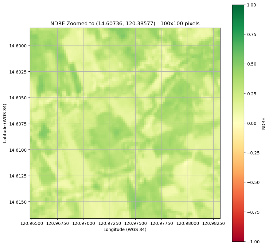
NDRE - Normalized Difference Red Edge

The Normalized Difference Red Edge (NDRE) index is a vegetation index used in remote sensing to assess the health and vitality of crops, particularly in more mature or stressed plants. It is similar to NDVI but utilizes the red-edge part of the spectrum, which is more sensitive to chlorophyll content and plant stress.

Applications of NDRE:

Crop Health Monitoring

Evaluates the health and vigor of crops, particularly in dense or mature vegetation where NDVI may be less effective. Nutrient Management: Helps detect nutrient deficiencies in plants, allowing for targeted fertilization strategies.

Precision Agriculture

Provides farmers with insights for optimizing irrigation and nutrient application based on plant stress levels.

Forestry Management

Assesses the health of forest canopies and helps monitor changes in forest ecosystems. Environmental Monitoring: Detects stress in vegetation caused by environmental changes, diseases, or pests, contributing to better land management practices.

\[NDRE = \frac{{\text{NIR} - \text{RE}}}{{\text{NIR} + \text{RE}}}\]

RE - shortwave infrared (Sentinel-2 - B05; also B06 and B07)

NIR - near-infrared band (Sentinel-2 - B08/B8A)

NDRE Value	Interpretation
+1	Very healthy vegetation with high chlorophyll content
0.6 to 0.9	Healthy vegetation, indicating good nutrient levels
0.2 to 0.5	Moderate vegetation health, possibly indicating stress
0.0 to 0.2	Poor vegetation health, indicating significant stress or nutrient deficiency
Below 0	Non-vegetated or very stressed areas

Calculate NDRE

• The script defines paths to Red Edge (RE) and Near-Infrared (NIR) bands within a Sentinel-2 .SAFE folder, using wildcards to locate files accurately.

• It loads these bands along with their Coordinate Reference System (CRS) and transformation details for geospatial alignment.

• NDRE is calculated by dividing the difference between NIR and Red bands by their sum, with a small constant added to avoid division by zero errors.

# Define paths to bands (inside your .SAFE folder)
base_folder = f"{name_download}/{name_download}/GRANULE"
red_edge_path_pattern = "*/IMG_DATA/R20m/*_B05_20m.jp2"
nir_path_pattern = "*/IMG_DATA/R20m/*_B8A_20m.jp2"

# Create a Path object
base_path = pathlib.Path(base_folder)

# Use rglob to find the actual file paths with wildcards
band_red_edge_path = next(base_path.rglob(red_edge_path_pattern), None)
band_nie_path = next(base_path.rglob(nir_path_pattern), None)

# Load the Red and Red Edge bands with their CRS and transformation
red_edge, red_edge_crs, red_edge_transform = load_band(band_red_edge_path)
nir, nir_crs, nir_transform = load_band(band_nie_path)

# Calculate NDRE
ndre = (nir.astype(float) - red_edge.astype(float)) / (nir + red_edge + 1e-10)

Reproject to WGS 84.

# Reproject NDRE to WGS 84 (EPSG:4326)
target_crs = 'EPSG:4326'
height, width = red.shape
bounds = rasterio.transform.array_bounds(height, width, red_transform)

# Calculate the transform and dimensions for the new projection
transform, width, height = calculate_default_transform(
    red_crs, target_crs, width, height, *bounds
)

# Prepare the NDVI array to be reprojected with the new shape
ndre_reprojected = np.empty((height, width), dtype=np.float32)

# Perform the reprojection into the new array
reproject(
    ndre,
    ndre_reprojected,
    src_transform=red_transform,
    src_crs=red_crs,
    dst_transform=transform,
    dst_crs=target_crs,
    resampling=Resampling.bilinear
)

(array([[0., 0., 0., ..., 0., 0., 0.],
        [0., 0., 0., ..., 0., 0., 0.],
        [0., 0., 0., ..., 0., 0., 0.],
        ...,
        [0., 0., 0., ..., 0., 0., 0.],
        [0., 0., 0., ..., 0., 0., 0.],
        [0., 0., 0., ..., 0., 0., 0.]], dtype=float32),
 Affine(0.00018313590139129615, 0.0, 120.20554290877753,
        0.0, -0.00018313590139129615, 15.375878870057374))

Clip image to the selected area.

# Define the coordinates to zoom into
latitude = 14.60736
longitude = 120.38577

# Get pixel coordinates for the target latitude and longitude
pixel_row, pixel_col = latlon_to_pixel(transform, latitude, longitude)

# Define the size of the zoom window (100x100 pixels around the point)
window_size = 100
row_start = max(0, pixel_row - window_size // 2)
row_end = min(height, pixel_row + window_size // 2)
col_start = max(0, pixel_col - window_size // 2)
col_end = min(width, pixel_col + window_size // 2)

# Crop the NDRE image to this window
ndre_zoomed = ndre_reprojected[row_start:row_end, col_start:col_end]

# Clip NDRE values to [-1, 1] for better visualization
ndre_zoomed = np.clip(ndre_zoomed, -1, 1)

# Calculate the new geographic bounds for the zoomed area
new_xmin = transform[2] + transform[0] * col_start + transform[1] * row_start  # Longitude min
new_xmax = transform[2] + transform[0] * col_end + transform[1] * row_start    # Longitude max
new_ymin = transform[5] + transform[4] * col_start + transform[3] * row_start  # Latitude min
new_ymax = transform[5] + transform[4] * col_end + transform[3] * row_end      # Latitude max
new_bounds = (new_xmin, new_xmax, new_ymin, new_ymax)

Plot an clipped image

plt.figure(figsize=(10, 10))

plt.imshow(ndre_zoomed, cmap='RdYlGn',
           extent=new_bounds,
           origin='upper', vmin=-1, vmax=1)  # Set vmin and vmax for color scaling

# Set axis limits to match the geographic extents
plt.xlim(new_bounds[0], new_bounds[1])
plt.ylim(new_bounds[2], new_bounds[3])

# Format the longitude axis to prevent scientific notation
plt.gca().xaxis.set_major_formatter(ticker.FuncFormatter(lambda x, _: f"{x:.5f}"))

# Add grid and colorbar for better visualization
plt.colorbar(label='NDRE')
plt.title(f"NDRE Zoomed to ({latitude}, {longitude}) - 100x100 pixels")
plt.xlabel('Longitude (WGS 84)')
plt.ylabel('Latitude (WGS 84)')
plt.grid(True)

# Show the plot
plt.show()

Summary

The notebook introduced how to use Sentinel-2 data to calculate some the most popular vegetation indices including NDVI, NDII and NDRE. It might be a starting point for further analysis, including extraction of the values from images, time series and monitoring of individual fields.

What To Do Next

To learn more about processing different types of satellite data, check the following articles:

• Air quality using Sentinel-5P data in JupyterLab on CopPhil

• Urban heat island monitoring using Sentinel-3 data in JupyterLab on CopPhil

• Using Sentinel-2 images to monitor mouth of the river Pampanga and Pampanga-Bay in JupyterLab on CopPhil