Air quality using Sentinel-5P data in JupyterLab on CopPhil
The following example aims to present how to interact with the catalogue, download EO data products and do some basic visualization regarding air quality. It is divided into five main parts:
Search for Sentinel-5P Level 2 products using specific filters
Download data
Process data using HARP
Create a map of nitrogen dioxide pollution (NO2) over the Philippines
Verify NO2 pollution over 10 most populated cities in Philippines
Prerequisites
No. 1 Access to CopPhil site
You need a CopPhil hosting account, available at https://infra.copphil.philsa.gov.ph.
No. 2 Access to JupyterLab
JupyterLab used in this article is available here: https://jupyter.infra.copphil.philsa.gov.ph/hub/login?next=%2Fhub%2F.
No. 3 Working knowledge of JupyterLab
See article Introduction to JupyterLab on CopPhil
No. 4 Using API
This is an introductory example of obtaining EODATA using API calls, in Python:
Download satellite data using API on CopPhil
No. 5 Information on Sentinel-5P mission
Page Sentinel-5P mission shows basic information on Sentinel-5P mission, which is used in this article as a source of information.
No. 6 Use Geo science kernel
Geo science kernel has preinstalled all of the Python libraries in this article:
Python 3 kernel and Geo science kernel in JupyterLab on CopPhil
What We Are Going To Do
Prepare your environment
Search for Sentinel-5P product
Build a query
Inspect results of the request
Download data
Authentication
Select product to be downloaded
Unpack data
Create a list of files’ names
Using HARP - Atmospheric Toolbox
Visualization
Map of NO2 TVCD - Philippines
Create a visualization
Values extraction
Map of NO2 TVCD - Manila
Summary
Prepare your environment
Upload necessary python libraries.
# HTTP requests
import requests

# JSON parser
import json


# data manipulation
import pandas as pd
import numpy as np

# image manipulation
import matplotlib.pyplot as plt
import numpy as np
import harp
import matplotlib.cm as cm
import geopandas as gpd

# file manipulation
import zipfile
import os
Search for Sentinel-5P products
Let’s start with obtaining some data. To learn the basics, see Prerequisites No. 4. However, in this article another set of data is going to be used.
Build a query
In order to find desired products, it is needed to determine some specific filters:
- collection_name
Sentinel-5P - product_type: L2_NO2__ (tropospheric vertical NO2 column)
- processing_mode
processing_mode = NRTI (Near Real Time)
- aoi
extent (coordinates) of the area of interest (WGS84)
- search_period_start
time range - start date
- search_period_end
time range - end date
# Base URL of the product catalogue
catalogue_odata_url = "https://catalogue.infra.copphil.philsa.gov.ph/odata/v1"

# Search parameters
collection_name = "SENTINEL-5P"
product_type = "L2__NO2___"
processing_mode = "NRTI"
aoi = "POLYGON((120.962986 14.598416, 120.995964 14.599182, 120.999658 14.563436, 120.960348 14.567522, 120.962986 14.598416))"
search_period_start = "2024-02-01T00:00:00.000Z"
search_period_end = "2024-02-10T00:00:00.000Z"

# Construct the OData query
search_query = f"{catalogue_odata_url}/Products?$filter=Collection/Name eq '{collection_name}' and Attributes/OData.CSC.StringAttribute/any(att:att/Name eq 'productType' and att/OData.CSC.StringAttribute/Value eq '{product_type}') and Attributes/OData.CSC.StringAttribute/any(att:att/Name eq 'processingMode' and att/OData.CSC.StringAttribute/Value eq '{processing_mode}') and OData.CSC.Intersects(area=geography'SRID=4326;{aoi}') and ContentDate/Start gt {search_period_start} and ContentDate/Start lt {search_period_end}"

# Print the formatted URL
print(search_query)
https://catalogue.infra.copphil.philsa.gov.ph/odata/v1/Products?$filter=Collection/Name eq 'SENTINEL-5P' and Attributes/OData.CSC.StringAttribute/any(att:att/Name eq 'productType' and att/OData.CSC.StringAttribute/Value eq 'L2__NO2___') and Attributes/OData.CSC.StringAttribute/any(att:att/Name eq 'processingMode' and att/OData.CSC.StringAttribute/Value eq 'NRTI') and OData.CSC.Intersects(area=geography'SRID=4326;POLYGON((120.962986 14.598416, 120.995964 14.599182, 120.999658 14.563436, 120.960348 14.567522, 120.962986 14.598416))') and ContentDate/Start gt 2024-02-01T00:00:00.000Z and ContentDate/Start lt 2024-02-10T00:00:00.000Z
Inspect results of the request
Show the number of found products which fit into filters requirements and get a list of names and id’s of images which fits the query.
response = requests.get(search_query).json()
result = pd.DataFrame.from_dict(response["value"])

id_list = []
for element in response['value']:
    id_value = element['Id']
    id_list.append(id_value)

for id in id_list:
    print(id)

name_list = []
for element in response['value']:
    name_value = element['Name']
    name_list.append(name_value)

for name in name_list:
    print(name)

print(f'Number of products which meets query filters: {len(result)}')
85d17702-27a8-4839-857c-6f6e717f738b
9d53743d-a99a-4305-9008-23bbaf27e844
81f9010a-e9a3-4c44-bdab-f24c4e6c7b0a
3f201d0d-43c9-44e8-8f08-7e072116aaac
374aa291-460a-49e0-af5a-35614a038015
37cc2da1-36c5-479d-adae-7ec0fcb74624
822dec6d-9c47-4ea4-a7f0-1fde44a103d3
b3632086-50b8-43cb-836e-1a7180e6263c
4006b09f-b5a0-4e06-bf9a-1e18ef628f1d
ff447a89-3aae-4ac9-9ab7-30ce2d6dbfc4
1f4e8441-8866-4252-9829-411bba49f676
S5P_NRTI_L2__NO2____20240202T051748_20240202T052248_32671_03_020600_20240202T060653.nc
S5P_NRTI_L2__NO2____20240204T044248_20240204T044748_32699_03_020600_20240204T052849.nc
S5P_NRTI_L2__NO2____20240205T042248_20240205T042748_32713_03_020600_20240205T051132.nc
S5P_NRTI_L2__NO2____20240205T060248_20240205T060748_32714_03_020600_20240205T065020.nc
S5P_NRTI_L2__NO2____20240207T052748_20240207T053248_32742_03_020600_20240207T061608.nc
S5P_NRTI_L2__NO2____20240201T053748_20240201T054248_32657_03_020600_20240201T062701.nc
S5P_NRTI_L2__NO2____20240202T052248_20240202T052748_32671_03_020600_20240202T061013.nc
S5P_NRTI_L2__NO2____20240203T050248_20240203T050748_32685_03_020600_20240203T054914.nc
S5P_NRTI_L2__NO2____20240206T054748_20240206T055248_32728_03_020600_20240206T063554.nc
S5P_NRTI_L2__NO2____20240208T050748_20240208T051248_32756_03_020600_20240208T055417.nc
S5P_NRTI_L2__NO2____20240209T044748_20240209T045248_32770_03_020600_20240209T053529.nc
Number of products which meets query filters: 11
Download data
Authentication
Log in to the portal. If status_code=200, it means you are logged successfully.
# Provide CopPhil account credentials - replace with your own data

username = 'username'
password = 'password'

auth_server_url = "https://auth.copphil.cloudferro.com/auth/realms/copphilinfra/protocol/openid-connect/token"
data = {
    "client_id": "copphil-public",
    "grant_type": "password",
    "username": username,
    "password": password,
}

response = requests.post(auth_server_url, data=data, verify=True, allow_redirects=False)
access_token = json.loads(response.text)["access_token"]
status_code = response.status_code
print(status_code)
200
Select product to be downloaded
From the list which was provided in the previous stage and based on image name and id, let’s download the proper images.
# Download each file using the IDs and corresponding names
for id_value, name_value in zip(id_list, name_list):
    # Construct the download URL for each file
    url_download = f'https://download.infra.copphil.philsa.gov.ph/odata/v1/Products({id_download})/$value'
    url_download_using_token = url_download + '?token=' + access_token

    # Download the file
    pulling = requests.get(url_download_using_token)

    # Save the file using the corresponding name
    with open(f"{name_value}.zip", 'wb') as file:
        file.write(pulling.content)

    print(f"Downloaded {name_value}.zip")
Downloaded S5P_NRTI_L2__NO2____20240202T051748_20240202T052248_32671_03_020600_20240202T060653.nc.zip
Downloaded S5P_NRTI_L2__NO2____20240204T044248_20240204T044748_32699_03_020600_20240204T052849.nc.zip
Downloaded S5P_NRTI_L2__NO2____20240205T042248_20240205T042748_32713_03_020600_20240205T051132.nc.zip
Downloaded S5P_NRTI_L2__NO2____20240205T060248_20240205T060748_32714_03_020600_20240205T065020.nc.zip
Downloaded S5P_NRTI_L2__NO2____20240207T052748_20240207T053248_32742_03_020600_20240207T061608.nc.zip
Downloaded S5P_NRTI_L2__NO2____20240201T053748_20240201T054248_32657_03_020600_20240201T062701.nc.zip
Downloaded S5P_NRTI_L2__NO2____20240202T052248_20240202T052748_32671_03_020600_20240202T061013.nc.zip
Downloaded S5P_NRTI_L2__NO2____20240203T050248_20240203T050748_32685_03_020600_20240203T054914.nc.zip
Downloaded S5P_NRTI_L2__NO2____20240206T054748_20240206T055248_32728_03_020600_20240206T063554.nc.zip
Downloaded S5P_NRTI_L2__NO2____20240208T050748_20240208T051248_32756_03_020600_20240208T055417.nc.zip
Downloaded S5P_NRTI_L2__NO2____20240209T044748_20240209T045248_32770_03_020600_20240209T053529.nc.zip
Unpack data
Unzip downloaded folders.
# Directory where the zip files are stored
download_directory = "."  # Change this to your specific directory if needed

# Iterate through all files in the specified directory
for filename in os.listdir(download_directory):
    if filename.endswith('.zip'):
        zip_file_path = os.path.join(download_directory, filename)

        # Create a directory to extract the contents into
        extract_directory = os.path.join(download_directory, os.path.splitext(filename)[0])

        # Append a timestamp if the directory already exists
        while os.path.exists(extract_directory):
            extract_directory = f"{extract_directory}_{int(time.time())}"

        # Create the directory
        os.makedirs(extract_directory, exist_ok=True)

        # Unzip the file
        try:
            with zipfile.ZipFile(zip_file_path, 'r') as zip_ref:
                zip_ref.extractall(extract_directory)

            print(f"Unzipped {filename} to {extract_directory}")
        except zipfile.BadZipFile:
            print(f"Error: {filename} is a corrupted zip file.")
        except Exception as e:
            print(f"An unexpected error occurred while unzipping {filename}: {e}")
    else:
        print(f"File {filename} is not a zip file. Skipping.")
Unzipped S5P_NRTI_L2__NO2____20240206T054748_20240206T055248_32728_03_020600_20240206T063554.nc.zip to ./S5P_NRTI_L2__NO2____20240206T054748_20240206T055248_32728_03_020600_20240206T063554.nc
Unzipped S5P_NRTI_L2__NO2____20240204T044248_20240204T044748_32699_03_020600_20240204T052849.nc.zip to ./S5P_NRTI_L2__NO2____20240204T044248_20240204T044748_32699_03_020600_20240204T052849.nc
Unzipped S5P_NRTI_L2__NO2____20240207T052748_20240207T053248_32742_03_020600_20240207T061608.nc.zip to ./S5P_NRTI_L2__NO2____20240207T052748_20240207T053248_32742_03_020600_20240207T061608.nc
Unzipped S5P_NRTI_L2__NO2____20240205T042248_20240205T042748_32713_03_020600_20240205T051132.nc.zip to ./S5P_NRTI_L2__NO2____20240205T042248_20240205T042748_32713_03_020600_20240205T051132.nc
File Air-quality-using-Sentinel-5P-data-in-JupyterLab-on-Eumetsat-Elasticity.rst is not a zip file. Skipping.
Unzipped S5P_NRTI_L2__NO2____20240203T050248_20240203T050748_32685_03_020600_20240203T054914.nc.zip to ./S5P_NRTI_L2__NO2____20240203T050248_20240203T050748_32685_03_020600_20240203T054914.nc
Unzipped S5P_NRTI_L2__NO2____20240202T051748_20240202T052248_32671_03_020600_20240202T060653.nc.zip to ./S5P_NRTI_L2__NO2____20240202T051748_20240202T052248_32671_03_020600_20240202T060653.nc
Unzipped S5P_NRTI_L2__NO2____20240201T053748_20240201T054248_32657_03_020600_20240201T062701.nc.zip to ./S5P_NRTI_L2__NO2____20240201T053748_20240201T054248_32657_03_020600_20240201T062701.nc
Unzipped S5P_NRTI_L2__NO2____20240208T050748_20240208T051248_32756_03_020600_20240208T055417.nc.zip to ./S5P_NRTI_L2__NO2____20240208T050748_20240208T051248_32756_03_020600_20240208T055417.nc
Unzipped S5P_NRTI_L2__NO2____20240209T044748_20240209T045248_32770_03_020600_20240209T053529.nc.zip to ./S5P_NRTI_L2__NO2____20240209T044748_20240209T045248_32770_03_020600_20240209T053529.nc
File Air-quality-and-urban-heat-monitoring-using-Sentinel-5P-and-Sentinel-3-data-in-JupyterLab.ipynb is not a zip file. Skipping.
Unzipped S5P_NRTI_L2__NO2____20240202T052248_20240202T052748_32671_03_020600_20240202T061013.nc.zip to ./S5P_NRTI_L2__NO2____20240202T052248_20240202T052748_32671_03_020600_20240202T061013.nc
Unzipped S5P_NRTI_L2__NO2____20240205T060248_20240205T060748_32714_03_020600_20240205T065020.nc.zip to ./S5P_NRTI_L2__NO2____20240205T060248_20240205T060748_32714_03_020600_20240205T065020.nc
Create a list of files’ names
Create a list of merged names of .nc files which have been downloaded.
# Directory to search for .nc files
search_directory = "."  # Change this to your specific directory if needed

# List to store the paths of .nc files
nc_file_list = []

# Walk through the directory
for root, dirs, files in os.walk(search_directory):
    for file in files:
        if file.endswith('.nc'):
            nc_file_path = os.path.join(root, file)
            nc_file_list.append(nc_file_path)

# Print the list of .nc files
print("List of .nc files:")
for nc_file in nc_file_list:
    print(nc_file)
List of .nc files:
./S5P_NRTI_L2__NO2____20240209T044748_20240209T045248_32770_03_020600_20240209T053529.nc/S5P_NRTI_L2__NO2____20240209T044748_20240209T045248_32770_03_020600_20240209T053529/S5P_NRTI_L2__NO2____20240209T044748_20240209T045248_32770_03_020600_20240209T053529.nc
./S5P_NRTI_L2__NO2____20240205T042248_20240205T042748_32713_03_020600_20240205T051132.nc/S5P_NRTI_L2__NO2____20240205T042248_20240205T042748_32713_03_020600_20240205T051132/S5P_NRTI_L2__NO2____20240205T042248_20240205T042748_32713_03_020600_20240205T051132.nc
./S5P_NRTI_L2__NO2____20240206T054748_20240206T055248_32728_03_020600_20240206T063554.nc/S5P_NRTI_L2__NO2____20240206T054748_20240206T055248_32728_03_020600_20240206T063554/S5P_NRTI_L2__NO2____20240206T054748_20240206T055248_32728_03_020600_20240206T063554.nc
./S5P_NRTI_L2__NO2____20240208T050748_20240208T051248_32756_03_020600_20240208T055417.nc/S5P_NRTI_L2__NO2____20240208T050748_20240208T051248_32756_03_020600_20240208T055417/S5P_NRTI_L2__NO2____20240208T050748_20240208T051248_32756_03_020600_20240208T055417.nc
./S5P_NRTI_L2__NO2____20240205T060248_20240205T060748_32714_03_020600_20240205T065020.nc/S5P_NRTI_L2__NO2____20240205T060248_20240205T060748_32714_03_020600_20240205T065020/S5P_NRTI_L2__NO2____20240205T060248_20240205T060748_32714_03_020600_20240205T065020.nc
./S5P_NRTI_L2__NO2____20240201T053748_20240201T054248_32657_03_020600_20240201T062701.nc/S5P_NRTI_L2__NO2____20240201T053748_20240201T054248_32657_03_020600_20240201T062701/S5P_NRTI_L2__NO2____20240201T053748_20240201T054248_32657_03_020600_20240201T062701.nc
./S5P_NRTI_L2__NO2____20240207T052748_20240207T053248_32742_03_020600_20240207T061608.nc/S5P_NRTI_L2__NO2____20240207T052748_20240207T053248_32742_03_020600_20240207T061608/S5P_NRTI_L2__NO2____20240207T052748_20240207T053248_32742_03_020600_20240207T061608.nc
./S5P_NRTI_L2__NO2____20240204T044248_20240204T044748_32699_03_020600_20240204T052849.nc/S5P_NRTI_L2__NO2____20240204T044248_20240204T044748_32699_03_020600_20240204T052849/S5P_NRTI_L2__NO2____20240204T044248_20240204T044748_32699_03_020600_20240204T052849.nc
./S5P_NRTI_L2__NO2____20240202T051748_20240202T052248_32671_03_020600_20240202T060653.nc/S5P_NRTI_L2__NO2____20240202T051748_20240202T052248_32671_03_020600_20240202T060653/S5P_NRTI_L2__NO2____20240202T051748_20240202T052248_32671_03_020600_20240202T060653.nc
./S5P_NRTI_L2__NO2____20240202T052248_20240202T052748_32671_03_020600_20240202T061013.nc/S5P_NRTI_L2__NO2____20240202T052248_20240202T052748_32671_03_020600_20240202T061013/S5P_NRTI_L2__NO2____20240202T052248_20240202T052748_32671_03_020600_20240202T061013.nc
./S5P_NRTI_L2__NO2____20240203T050248_20240203T050748_32685_03_020600_20240203T054914.nc/S5P_NRTI_L2__NO2____20240203T050248_20240203T050748_32685_03_020600_20240203T054914/S5P_NRTI_L2__NO2____20240203T050248_20240203T050748_32685_03_020600_20240203T054914.nc
Using HARP - Atmospheric Toolbox
The HARP (Harmonized Atmospheric Retrieval Package) is an open-source software toolkit developed for processing and analyzing atmospheric composition data. It provides tools for data ingestion, filtering, resampling, and conversion, which make it particularly useful for harmonizing data from various atmospheric sensors and satellite instruments.
- A
The number of latitude edge points, calculates as follows: (N latitude of AoI (55) - S latitude of AOI (49) / C (0.01)) + 1
- S
The latitude offset at which to start the grid (S)
- SR
The spatial resolution expressed in degrees
- B
The number of longitude edge points, calculates as follows: (E longitude of AoI (25) - W longitude of AOI (14) / C (0.01)) + 1
- W
The longitude offset at which to start the grid (W)
- SR
The spatial resolution expressed in degrees
N = 21.00
S = 4.00
W = 116.00
E = 127.00

SR = 0.01

A = (N-S)/SR + 1
B = (E-W)/SR + 1

operations = ";".join([
    "tropospheric_NO2_column_number_density_validity>75",             # Keep pixels wich qa_value > 0.75
    "derive(surface_wind_speed {time} [m/s])",                        # Get surafe wind speed expressed in [m/s]
    "surface_wind_speed<5",                                           # Keep pixels wich wind_spped < 5 [m/s]
    # Keep variables defined below
    "keep(latitude_bounds,longitude_bounds,datetime_start,datetime_length,tropospheric_NO2_column_number_density, surface_wind_speed)",
    "derive(datetime_start {time} [days since 2000-01-01])",          # Get start time of the acquisition
    "derive(datetime_stop {time}[days since 2000-01-01])",            # Get end time of the acquisition
    "exclude(datetime_length)",                                       # Exclude datetime lenght
    f"bin_spatial({int(A)},{int(S)},{float(SR)},{int(B)},{int(W)},{float(SR)})",                       # Define bin spatial (details below)
    "derive(tropospheric_NO2_column_number_density [Pmolec/cm2])",    # Convert the NO2 units to 10^15 molec/cm^2
    "derive(latitude {latitude})",                                    # Get latitude
    "derive(longitude {longitude})",                                  # Get longitude
    "count>0"
])
Operations for temporal averaging.
reduce_operations=";".join([
    "squash(time, (latitude, longitude, latitude_bounds, longitude_bounds))",
    "bin()"
])
Create new image - average NO2 pollution over defined area in a specific period.
mean_no2 = harp.import_product(nc_file_list, operations, reduce_operations=reduce_operations)
Import and write new created image as a netcdf named “mean_no2_2024_02_01_10.nc”.
harp.export_product(mean_no2, 'mean_no2_2024_02_01_10.nc')
Visualization
Map of NO2 TVCD - Philippines
Select data related to nitrogen dioxide (NO2) pollution from the mean_no2 object. First, it retrieves the values for the tropospheric column number density of NO2 from the first time step, if applicable. Then, it extracts the description of the variable, which includes the name of the measurement, along with the units in which it is expressed.
# Select NO2 pollution
no2 = mean_no2.tropospheric_NO2_column_number_density.data[0, :, :]  # Select the first time step (if applicable)

# Select description (name) of variable
no2_description = mean_no2.tropospheric_NO2_column_number_density.description

# Select units of variable
no2_units = mean_no2.tropospheric_NO2_column_number_density.unit
Create a visualization
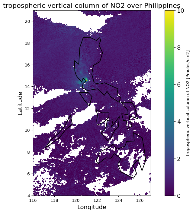
Visualize nitrogen dioxide (NO2) pollution levels over the Philippines.
# Define coordinates grid
gridlat = mean_no2.latitude_bounds.data[:, 0]  # First column (Southern bounds)
gridlon = mean_no2.longitude_bounds.data[:, 0]  # First column (Western bounds)

# Create a meshgrid for plotting
lon_edges = np.concatenate((gridlon, [gridlon[-1] + (gridlon[1] - gridlon[0])]))  # Extend the longitude bounds
lat_edges = np.concatenate((gridlat, [gridlat[-1] + (gridlat[1] - gridlat[0])]))  # Extend the latitude bounds

# Define legend
colortable = cm.viridis
vmin = 0
vmax = 10

# Load the world borders dataset
world = gpd.read_file(gpd.datasets.get_path('naturalearth_lowres'))

# Filter for the Philippines
philippines = world[world.name == "Philippines"]

# Create the plot
plt.figure(figsize=(12, 8))  # Set the figure size
plt.pcolormesh(lon_edges, lat_edges, no2, shading='auto', cmap=colortable, vmin=vmin, vmax=vmax)

# Add color bar
cbar = plt.colorbar(label=f'{no2_description} [{no2_units}]')
cbar.ax.tick_params(labelsize=14)

# Set titles and labels
plt.title(f'{no2_description} over Philippines', fontsize=16)
plt.xlabel('Longitude', fontsize=14)
plt.ylabel('Latitude', fontsize=14)

# Add the borders of the Philippines
philippines.boundary.plot(ax=plt.gca(), color='black', linewidth=1.5)

# Show the plot
plt.show()
/tmp/ipykernel_457858/3501187648.py:15: FutureWarning: The geopandas.dataset module is deprecated and will be removed in GeoPandas 1.0. You can get the original 'naturalearth_lowres' data from https://www.naturalearthdata.com/downloads/110m-cultural-vectors/.
  world = gpd.read_file(gpd.datasets.get_path('naturalearth_lowres'))
Values extraction
Extract values of NO2 TVCD over 10 most populated cities in Philippines and plot results.
# List of the ten largest cities in the Philippines with their coordinates
cities = {
    'Quezon City': (14.6760, 121.0437),
    'Manila': (14.5995, 120.9842),
    'Caloocan': (14.6500, 120.9667),
    'Davao City': (7.1907, 125.4553),
    'Cebu City': (10.3157, 123.8854),
    'Zamboanga City': (6.8922, 122.0877),
    'Antipolo': (14.5807, 121.1135),
    'Pasig City': (14.5825, 121.0597),
    'Taguig City': (14.5285, 121.0555),
    'Iloilo City': (10.6910, 122.5641)
}

# Select NO2 pollution data
no2_data = mean_no2.tropospheric_NO2_column_number_density.data

# Define an empty dictionary to store NO2 values for each city
city_no2_values = {}

# Loop through each city and extract NO2 values
for city, (lat, lon) in cities.items():
    # Find the nearest indices in the grid
    lat_idx = np.abs(mean_no2.latitude_bounds.data[:, 0] - lat).argmin()
    lon_idx = np.abs(mean_no2.longitude_bounds.data[:, 0] - lon).argmin()

    # Extract NO2 value for the city
    city_no2_values[city] = no2_data[:, lat_idx, lon_idx]  # Assuming time is the first dimension

# Convert to DataFrame for better visualization
no2_df = pd.DataFrame(city_no2_values)

# Transpose the DataFrame to have cities as rows
no2_df = no2_df.T

# Set the column names to indicate the time steps (if applicable)
no2_df.columns = [f'NO2' for i in range(no2_data.shape[0])]

# Round the values to 2 decimal places
no2_df = no2_df.round(2)

# Calculate the mean NO2 value for sorting
no2_df['Average NO2'] = no2_df.mean(axis=1)

# Sort by the Average NO2 value in descending order
no2_df_sorted = no2_df.sort_values(by='Average NO2', ascending=False)

# Drop the Average NO2 column for final display
no2_df_sorted = no2_df_sorted.drop(columns='Average NO2')

# Display the results in a table
print(f"NO2 Pollution Levels in the Ten Largest Cities in the Philippines (in units of {no2_units}):")
print(no2_df_sorted)
NO2 Pollution Levels in the Ten Largest Cities in the Philippines (in units of Pmolec/cm2):
                  NO2
Taguig City     10.82
Manila           9.79
Pasig City       7.61
Caloocan         7.53
Quezon City      4.21
Antipolo         3.57
Iloilo City      1.19
Cebu City        1.13
Zamboanga City   0.41
Davao City       0.28
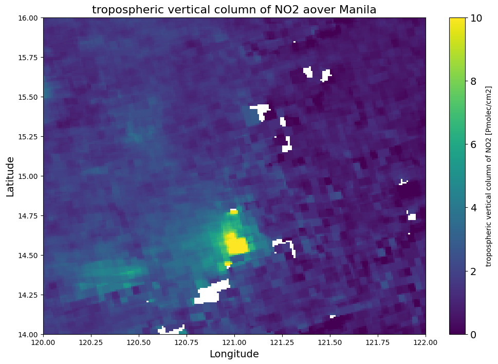
Map of NO2 TVCD - Manila
Define variable, longitude, latitude and colormap which are going to be visualized - limited to Manila
Area of interest - Manila
N = 16.00 S = 14.00 W = 120.00 E = 122.00
N = 16.00
S = 14.00
W = 120.00
E = 122.00

# Define coordinates grid
gridlat = mean_no2.latitude_bounds.data[:, 0]  # First column (Southern bounds)
gridlon = mean_no2.longitude_bounds.data[:, 0]  # First column (Western bounds)

# Create a meshgrid for plotting
lon_edges = np.concatenate((gridlon, [gridlon[-1] + (gridlon[1] - gridlon[0])]))  # Extend the longitude bounds
lat_edges = np.concatenate((gridlat, [gridlat[-1] + (gridlat[1] - gridlat[0])]))  # Extend the latitude bounds

# Define legend
colortable = cm.viridis
vmin = 0
vmax = 10

# Create the plot
plt.figure(figsize=(12, 8))  # Set the figure size
plt.pcolormesh(lon_edges, lat_edges, no2, shading='auto', cmap=colortable, vmin=vmin, vmax=vmax)

# Add color bar
cbar = plt.colorbar(label=f'{no2_description} [{no2_units}]')
cbar.ax.tick_params(labelsize=14)

# Set titles and labels
plt.title(f'{no2_description} aover Manila', fontsize=16)
plt.xlabel('Longitude', fontsize=14)
plt.ylabel('Latitude', fontsize=14)

# Set extent to the specified boundaries
plt.xlim(W, E)
plt.ylim(S, N)

# Show the plot
plt.show()
Summary
With the proposed tutorial you can easily and effectively process huge amounts of Sentinel-5P data starting with defining specific datasets, through processing with the HARP toolbox, ending with creating and writing new data.
What To Do Next
To learn more about processing different types of satellite data, check the following articles: