Using Sentinel-2 images to monitor mouth of the river Pampanga and Pampanga-Bay in JupyterLab on CopPhil
In this notebook, you learn how to access data from CopPhil using API and what you can do with it. As an example, we will try to access Sentinel-2 images containing data of Pampanga river and Pampanga Bay, from January to June 2023. With usage of few Python packages, you will be able to obtain images with Normalized difference Water Index (NDWI).
We will focus on monitoring quantity of water in the area of Pampanga river’s mouth.
Prerequisites
No. 1 Access to CopPhil site
You need a CopPhil hosting account, available at https://infra.copphil.philsa.gov.ph.
No. 2 Access to JupyterLab
JupyterLab used in this article is available here: https://jupyter.infra.copphil.philsa.gov.ph/hub/login?next=%2Fhub%2F.
No. 3 Working knowledge of JupyterLab
For general information on using JupyterLab environment, see Introduction to JupyterLab on CopPhil
No. 4 Using API
This is an introductory example of obtaining EODATA using API calls, in Python:
Download satellite data using API on CopPhil
No. 5 Information on Sentinel-2 mission
Page Sentinel-2 mission shows basic information on Sentinel-2 mission, which is used in this article as a source of information.
What We Are Going To Do
Prepare your environment
Search for Sentinel-2 L2A products
Build a query
Inspect results of the request
Download data
Authentication
Download multiple files
Unpack data
Calculating NDWI
Functions for reading, calculating and saving raster data
Define images to be processed
Computing NWDI rasters
Visualization
Visualization - colormap
Visualization - water/no-water classification
Summary
Prepare your environment
Upload necessary python libraries.
# HTTP requests
import requests

# JSON parser
import json

# data manipulation
import pandas as pd
import numpy as np

# image manipulation
import rasterio
from rasterio.plot import show
import matplotlib.pyplot as plt
import matplotlib.patches as patches
from osgeo import gdal, gdal_array, osr

# file manipulation
import zipfile
import os
Search for Sentinel-2 L2A products
Let’s start with obtaining some data.
Build a query
In order to find desired products it is needed to determinate the following filters:
- collection_name:
Sentinel-2
- product_type:
MSIL2A
- aoi
extent (coordinates) of the area of interest (WGS84)
- search_period_start
time range - start date
- search_period_end
time range - end date
- max_cloud_cover
maximum cloud cover (%) fo the image
# base URL of the product catalogue
catalogue_odata_url = "https://catalogue.infra.copphil.philsa.gov.ph/odata/v1"

# search parameters
collection_name = "SENTINEL-2"
product_type = "S2MSI2A"
aoi = "POLYGON((120.962986 14.598416, 120.995964 14.599182, 120.999658 14.563436, 120.960348 14.567522, 120.962986 14.598416))"
search_period_start = "2023-01-01T00:00:00.000Z"
search_period_end = "2023-07-30T00:00:00.000Z"

search_query = f"{catalogue_odata_url}/Products?$filter=Collection/Name eq '{collection_name}' and Attributes/OData.CSC.StringAttribute/any(att:att/Name eq 'productType' and att/OData.CSC.StringAttribute/Value eq '{product_type}') and OData.CSC.Intersects(area=geography'SRID=4326;{aoi}') and ContentDate/Start gt {search_period_start} and ContentDate/Start lt {search_period_end}"

max_cloud_cover = 20

search_query_cloud = f"{search_query} and Attributes/OData.CSC.DoubleAttribute/any(att:att/Name eq 'cloudCover' and att/OData.CSC.DoubleAttribute/Value le {max_cloud_cover})"
print(f"""\n{search_query.replace(' ', "%20")}\n""")
https://catalogue.infra.copphil.philsa.gov.ph/odata/v1/Products?$filter=Collection/Name%20eq%20'SENTINEL-2'%20and%20Attributes/OData.CSC.StringAttribute/any(att:att/Name%20eq%20'productType'%20and%20att/OData.CSC.StringAttribute/Value%20eq%20'S2MSI2A')%20and%20OData.CSC.Intersects(area=geography'SRID=4326;POLYGON((120.962986%2014.598416,%20120.995964%2014.599182,%20120.999658%2014.563436,%20120.960348%2014.567522,%20120.962986%2014.598416))')%20and%20ContentDate/Start%20gt%202023-01-01T00:00:00.000Z%20and%20ContentDate/Start%20lt%202023-07-30T00:00:00.000Z
Inspect results of the request
Show the number of found products which fits into filters requirements and get a list of names and id’s of images which fits the query.
response = requests.get(search_query_cloud).json()
result = pd.DataFrame.from_dict(response["value"])

id_list = []
for element in response['value']:
    id_value = element['Id']  # Get the Id value
    id_list.append(id_value)  # Append it to the list

for id in id_list:
    print(id)

name_list = []
for element in response['value']:
    name_value = element['Name']  # Get the Id value
    name_list.append(name_value)  # Append it to the list

for name in name_list:
    print(name)

print(f'Number of products which meets query filters: {len(result)}')
4f37ba0e-4f74-5f8f-87e5-42efb1a2130e
d9ef8789-9d93-510a-aade-d72d35bb94ce
b8373f23-0ee8-48cb-aa08-9bbbf4c51f30
8c7fc594-cc21-47e2-8588-77772969ffd5
cbf2bf2d-5707-49e0-bf54-23fdb652872d
S2B_MSIL2A_20230107T022059_N0509_R003_T51PTS_20230107T051542.SAFE
S2A_MSIL2A_20230201T021921_N0509_R003_T51PTS_20230201T052000.SAFE
S2A_MSIL2A_20230323T021531_N0509_R003_T51PTS_20230323T070005.SAFE
S2B_MSIL2A_20230706T021539_N0509_R003_T51PTS_20230706T052627.SAFE
S2B_MSIL2A_20230507T021539_N0509_R003_T51PTS_20230507T043713.SAFE
Number of products which meets query filters: 5
Download data
Authentication
Log in to the portal. If status_code=200, it means you are logged successfully.
# Provide CopPhil account credentials - replace with your own data

username = 'username'
password = 'password'

auth_server_url = "https://auth.copphil.cloudferro.com/auth/realms/copphilinfra/protocol/openid-connect/token"
data = {
    "client_id": "copphil-public",
    "grant_type": "password",
    "username": username,
    "password": password,
}

response = requests.post(auth_server_url, data=data, verify=True, allow_redirects=False)
access_token = json.loads(response.text)["access_token"]
status_code = response.status_code
print(status_code)
200
Download multiple files
From the list which was provided in the previous stage and based on image name and id, let’s download the proper images.
# Download each file using the IDs and corresponding names
for id_value, name_value in zip(id_list, name_list):
    # Construct the download URL for each file
    url_download = f'https://download.infra.copphil.philsa.gov.ph/odata/v1/Products({id_download})/$value'
    url_download_using_token = url_download + '?token=' + access_token

    # Download the file
    pulling = requests.get(url_download_using_token)

    # Save the file using the corresponding name
    with open(f"{name_value}.zip", 'wb') as file:
        file.write(pulling.content)

    print(f"Downloaded {name_value}.zip")
Downloaded S2B_MSIL2A_20230107T022059_N0509_R003_T51PTS_20230107T051542.SAFE.zip
Downloaded S2A_MSIL2A_20230201T021921_N0509_R003_T51PTS_20230201T052000.SAFE.zip
Downloaded S2A_MSIL2A_20230323T021531_N0509_R003_T51PTS_20230323T070005.SAFE.zip
Downloaded S2B_MSIL2A_20230706T021539_N0509_R003_T51PTS_20230706T052627.SAFE.zip
Downloaded S2B_MSIL2A_20230507T021539_N0509_R003_T51PTS_20230507T043713.SAFE.zip
Unpack data
Unzip downloaded folders.
# Directory where the zip files are stored
download_directory = "."  # Change this to your specific directory if needed

# Iterate through all files in the specified directory
for filename in os.listdir(download_directory):
    if filename.endswith('.zip'):  # Check if the file is a ZIP file
        zip_file_path = os.path.join(download_directory, filename)

        # Create a directory to extract the contents into
        extract_directory = os.path.join(download_directory, os.path.splitext(filename)[0])

        # Append a timestamp if the directory already exists
        while os.path.exists(extract_directory):
            extract_directory = f"{extract_directory}_{int(time.time())}"

        # Create the directory
        os.makedirs(extract_directory, exist_ok=True)

        # Unzip the file
        try:
            with zipfile.ZipFile(zip_file_path, 'r') as zip_ref:
                zip_ref.extractall(extract_directory)

            print(f"Unzipped {filename} to {extract_directory}")
        except zipfile.BadZipFile:
            print(f"Error: {filename} is a corrupted zip file.")
        except Exception as e:
            print(f"An unexpected error occurred while unzipping {filename}: {e}")
    else:
        print(f"File {filename} is not a zip file. Skipping.")
Unzipped S2B_MSIL2A_20230507T021539_N0509_R003_T51PTS_20230507T043713.SAFE.zip to ./S2B_MSIL2A_20230507T021539_N0509_R003_T51PTS_20230507T043713.SAFE
File Using-Sentinel-2-images-to-monitor-mouth-of-the-river-Pampanga-and-Pampanga-Bay-in-JupyterLab-on-Eumetsat-Elasticity.rst is not a zip file. Skipping.
Unzipped S2A_MSIL2A_20230323T021531_N0509_R003_T51PTS_20230323T070005.SAFE.zip to ./S2A_MSIL2A_20230323T021531_N0509_R003_T51PTS_20230323T070005.SAFE
Unzipped S2B_MSIL2A_20230107T022059_N0509_R003_T51PTS_20230107T051542.SAFE.zip to ./S2B_MSIL2A_20230107T022059_N0509_R003_T51PTS_20230107T051542.SAFE
Unzipped S2A_MSIL2A_20230201T021921_N0509_R003_T51PTS_20230201T052000.SAFE.zip to ./S2A_MSIL2A_20230201T021921_N0509_R003_T51PTS_20230201T052000.SAFE
File Using -Sentinel-2-images-to-monitor-mouth-of-the-river-Pampanga-and-Pampanga-Bay.ipynb is not a zip file. Skipping.
Unzipped S2B_MSIL2A_20230706T021539_N0509_R003_T51PTS_20230706T052627.SAFE.zip to ./S2B_MSIL2A_20230706T021539_N0509_R003_T51PTS_20230706T052627.SAFE
Calculating NDWI
Raster images containing the NDWI indicator can be used in various fields, including:
- Water Resource Monitoring
Tracking changes in water levels in lakes, rivers, and reservoirs, especially important in areas affected by drought or excessive rainfall. *
- Crisis Management
Rapid identification of flooded areas during floods and assessment of damages.
Environmental Protection
Monitoring wetlands and other aquatic ecosystems to preserve their biodiversity.
- Urban Planning
Analyzing the impact of urban development on nearby water resources.
- Agriculture
Assessing irrigation of agricultural fields and monitoring plant health.
NDWI is a normalized difference index calculated based on the reflectance of light in two different spectral bands: green (G) and near-infrared (NIR). The formula for calculating NDWI is as follows:
- G
Reflectance in the green band
- NIR
Reflectance in the near-infrared band.
NDWI values range from -1 to 1, where higher values indicate the presence of water, while the lower values may indicate other land cover types, such as vegetation or urban areas.
Functions for reading, calculating and saving raster data
Here we present you some functions for reading raster data into Numpy matrix, calculating NDWI with NIR and GREEN matrices and saving result as a new raster. We will conduct such calculation for each downloaded item. In the end, we will obtain NDWI data on Pampanga Bay area from a period of five months - from January to May 2024.
def getFullPath(dir: str, resolution: int, band: str):
    if not os.path.isdir(dir):
        raise ValueError(f"Provided path does not exist: {dir}")
    elif resolution not in [10,20,60]:
        raise ValueError(f"Provided resolution does not exist: R{resolution}m")
    else:
        full_path = dir
        while True:
            content = os.listdir(full_path)
            if len(content) == 0:
                raise ValueError(f"Directory empty: {full_path}")
            elif len(content) == 1:
                if full_path[-1] != '/':
                    full_path = full_path + '/' + content[0]
                else:
                    full_path = full_path + content[0]
            else:
                if 'GRANULE' in content:
                    full_path = full_path + '/' + 'GRANULE'
                    break
                else:
                    raise ValueError(f"Unsupported dir architecture: {full_path}")
        full_path = full_path + '/' + os.listdir(full_path)[0]
        full_path = full_path + '/' + "IMG_DATA"
        if len(os.listdir(full_path)) == 3:
            full_path = full_path + '/' + f'R{resolution}m'
            images = os.listdir(full_path)
            for img in images:
                if band in img:
                    return full_path + '/' + img
            raise ValueError(f'No such band {band} in directory: {full_path}')
        else:
            images = os.listdir(full_path)
            for img in images:
                if band in img:
                    return full_path + '/' + img
            raise ValueError(f'No such band {band} in directory: {full_path}')

# Get transformation matrix from raster
def getTransform(pathToRaster):
    dataset = gdal.Open(pathToRaster)
    transformation = dataset.GetGeoTransform()
    return transformation

# Read raster and return pixels' values matrix as int16, new transformation matrix, crs
def readRaster(path, resolution, band):
    path = getFullPath(path, resolution, band)
    trans = getTransform(path) # trzeba zdefiniować który kanał
    raster, crs = rasterToMatrix(path)
    return raster.astype(np.int16), crs, trans

def rasterToMatrix(pathToRaster):
    with rasterio.open(pathToRaster) as src:
        matrix = src.read(1)
    return matrix, src.crs.to_epsg()

# Transform numpy's matrix to geotiff; pass new raster's filepath, matrix with pixels' values, gdal file type, transformation matrix, projection, nodata value
def npMatrixToGeotiff(filepath, matrix, gdalType, projection, transformMatrix, nodata = None):
    driver = gdal.GetDriverByName('Gtiff')
    if len(matrix.shape) > 2:
        (bandNr, yRes, xRes) = matrix.shape
        image = driver.Create(filepath, xRes, yRes, bandNr, gdalType)
        for b in range(bandNr):
            b = b + 1
            band = image.GetRasterBand(b)
            if nodata is not None:
                band.SetNoDataValue(nodata)
            band.WriteArray(matrix[b-1,:,:])
            band.FlushCache
    else:
        bandNr = 1
        (yRes, xRes) = matrix.shape
        image = driver.Create(filepath, xRes, yRes, bandNr, gdalType)
        print(type(image))
        band = image.GetRasterBand(bandNr)
        if nodata is not None:
            band.SetNoDataValue(nodata)
        band.WriteArray(matrix)
        band.FlushCache
    image.SetGeoTransform(transformMatrix)
    image.SetProjection(projection)
    del driver, image, band
Define images to be processed
Create a list of images which are going to be processed.
# Directory to search for .SAFE directories
search_directory = "."  # Change this to your specific directory if needed

# List to store the paths of .SAFE directories
dataset_list = []

# List the contents of the search directory
for item in os.listdir(search_directory):
    item_path = os.path.join(search_directory, item)
    # Check if it is a directory and ends with .SAFE
    if os.path.isdir(item_path) and item.endswith('.SAFE'):
        dataset_list.append(item_path)

# Print the list of .SAFE directories
print("List of .SAFE directories:")
for dataset in dataset_list:
    print(dataset)
List of .SAFE directories:
./S2B_MSIL2A_20230706T021539_N0509_R003_T51PTS_20230706T052627.SAFE
./S2A_MSIL2A_20230201T021921_N0509_R003_T51PTS_20230201T052000.SAFE
./S2A_MSIL2A_20230323T021531_N0509_R003_T51PTS_20230323T070005.SAFE
./S2B_MSIL2A_20230107T022059_N0509_R003_T51PTS_20230107T051542.SAFE
./S2B_MSIL2A_20230507T021539_N0509_R003_T51PTS_20230507T043713.SAFE
Computing NWDI rasters
We will now use functions define above to generate NWDI rasters. The only data needed in this step, is a list of paths to our products (extracted from a zip archive). Function readRaster will select the specified band from the specified path.
#Path to catalog for processed images with NDWI index
compution_output = 'output'

# Iterating over single product
for item in dataset_list:
    # Reading name from path
    name = item.split('/')[-1]
    # Reading green band into matrix
    green = readRaster(item, 10, 'B03')
    # Reading NIR band into matrix
    nir = readRaster(item, 10, 'B08')
    # Calculating NDWI matrix
    ndwi = (green[0]-nir[0]) / (green[0]+nir[0])
    # Creating SpatialReference object and setting it to match original's raster CRS
    projection = osr.SpatialReference()
    projection.ImportFromEPSG(green[1])
    # Creating raster from matrix in GeoTiff format
    npMatrixToGeotiff(f'{compution_output}/{name}.tif', ndwi, gdal_array.NumericTypeCodeToGDALTypeCode(np.float32), projection.ExportToWkt(), green[2])
<class 'osgeo.gdal.Dataset'>
<class 'osgeo.gdal.Dataset'>
<class 'osgeo.gdal.Dataset'>
<class 'osgeo.gdal.Dataset'>
/tmp/ipykernel_1481986/3944644538.py:13: RuntimeWarning: invalid value encountered in divide
  ndwi = (green[0]-nir[0]) / (green[0]+nir[0])
<class 'osgeo.gdal.Dataset'>
Visualization
After successfully creating and saving new images, we can visualize them in Python, using rasterio package.
Firstly, try with the simplest example in order to verify if NDWI was calculated and images created.
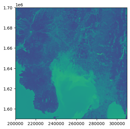
img = rasterio.open('output/S2A_MSIL2A_20230201T021921_N0509_R003_T51PTS_20230201T052000.SAFE.tif')
from rasterio.plot import show
show(img)
<Axes: >
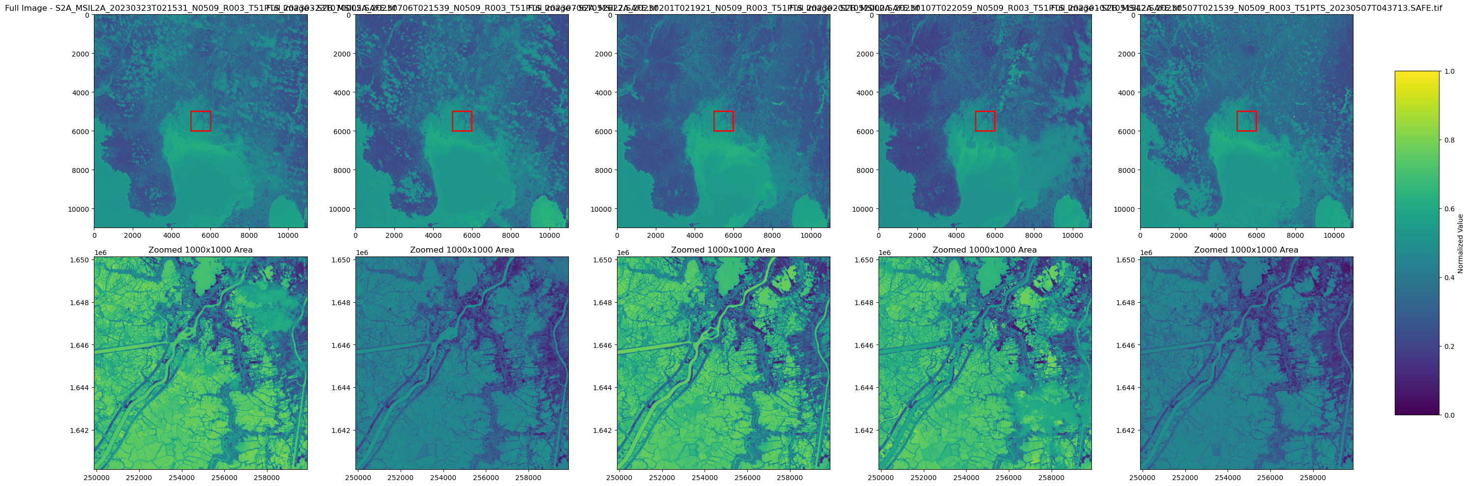
Visualization - colormap
- Directory Setup
Searches for .tif files in the specified directory output.
- Figure and Subplot Configuration
Creates a subplot grid with 2 rows and a dynamic number of columns based on file count; top row for full images, bottom row for zoomed areas.
- Image Loading and Normalization
Loads each .tif file, calculates normalization of image data (avoiding NaNs).
- Full Image Display
Shows the entire image with a viridis colormap and a red rectangle indicating the zoomed area.
- Zoomed Image Display
Displays a 1000x1000 pixel area centered within each image.
- Global Colorbar
Adds a colorbar scaled to the global min and max across all images.
- Layout Adjustments
Ensures the layout fits all subplots and the colorbar without overlap.
# Directory to search for .tif files
search_directory = "output"

# Collect all .tif files in the specified directory
tif_files = [os.path.join(search_directory, f) for f in os.listdir(search_directory) if f.endswith('.tif')]

# Set up a row of subplots with 2 rows for each image (one for full image, one for zoomed view)
num_files = len(tif_files)
fig, axes = plt.subplots(2, num_files, figsize=(6 * num_files, 10))

# Store the normalized data for colorbar scaling
all_img_data = []

# Plot each .tif file in separate subplots
for idx, tif_file in enumerate(tif_files):
    with rasterio.open(tif_file) as img:
        # Calculate center coordinates
        center_x, center_y = img.width // 2, img.height // 2

        # Define the bounds for a 1000x1000 pixel window around the center
        window = ((center_y - 500, center_y + 500), (center_x - 500, center_x + 500))

        # Plot the full image in the top row
        ax_full = axes[0, idx] if num_files > 1 else axes[0]
        img_data = img.read(1)

        # Check data range
        min_val = img_data.min()
        max_val = img_data.max()
        print(f"File: {os.path.basename(tif_file)} - Min: {min_val}, Max: {max_val}")

        # Handle no-data values (if applicable)
        no_data = img.nodata
        if no_data is not None:
            img_data = np.where(img_data == no_data, np.nan, img_data)

        # Normalize the image data for better display, avoiding NaN values
        img_data_normalized = (img_data - np.nanmin(img_data)) / (np.nanmax(img_data) - np.nanmin(img_data))
        all_img_data.append(img_data_normalized)

        # Show the normalized image with Viridis colormap
        show(img_data_normalized, ax=ax_full, cmap='viridis')
        ax_full.set_title(f"Full Image - {os.path.basename(tif_file)}")

        # Set axis limits to ensure the image is fully displayed
        ax_full.set_xlim(0, img.width)
        ax_full.set_ylim(img.height, 0)

        # Draw a rectangle to highlight the zoomed area in pixel coordinates
        rect = patches.Rectangle((center_x - 500, center_y - 500), 1000, 1000,
                                 linewidth=2, edgecolor='red', facecolor='none')

        ax_full.add_patch(rect)  # Add rectangle to the full image

        # Plot the zoomed 1000x1000 area in the bottom row
        img_array = img.read(1, window=window)

        # Normalize the zoomed image data for display, avoiding NaN values
        img_array = (img_array - np.nanmin(img_array)) / (np.nanmax(img_array) - np.nanmin(img_array))

        ax_zoom = axes[1, idx] if num_files > 1 else axes[1]
        show(img_array, ax=ax_zoom, transform=img.window_transform(window), cmap='viridis')
        ax_zoom.set_title("Zoomed 1000x1000 Area")

# Create a colorbar for the first subplot (representing the full image)
cbar_ax = fig.add_axes([0.91, 0.15, 0.03, 0.7])  #
vmin = min([np.nanmin(data) for data in all_img_data])
vmax = max([np.nanmax(data) for data in all_img_data])
cbar = plt.colorbar(plt.cm.ScalarMappable(cmap='viridis', norm=plt.Normalize(vmin=vmin, vmax=vmax)), cax=cbar_ax)
cbar.set_label('Normalized Value')

plt.tight_layout(rect=[0, 0, 0.9, 1])
plt.show()
File: S2A_MSIL2A_20230323T021531_N0509_R003_T51PTS_20230323T070005.SAFE.tif - Min: -1.0, Max: 1.0
File: S2B_MSIL2A_20230706T021539_N0509_R003_T51PTS_20230706T052627.SAFE.tif - Min: -1.0, Max: 1.0
File: S2A_MSIL2A_20230201T021921_N0509_R003_T51PTS_20230201T052000.SAFE.tif - Min: -1.0, Max: 1.0
File: S2B_MSIL2A_20230107T022059_N0509_R003_T51PTS_20230107T051542.SAFE.tif - Min: -0.8986014127731323, Max: 1.0
File: S2B_MSIL2A_20230507T021539_N0509_R003_T51PTS_20230507T043713.SAFE.tif - Min: nan, Max: nan
/tmp/ipykernel_1481986/2200105399.py:72: UserWarning: This figure includes Axes that are not compatible with tight_layout, so results might be incorrect.
  plt.tight_layout(rect=[0, 0, 0.9, 1])  # Adjust layout to make room for colorbar
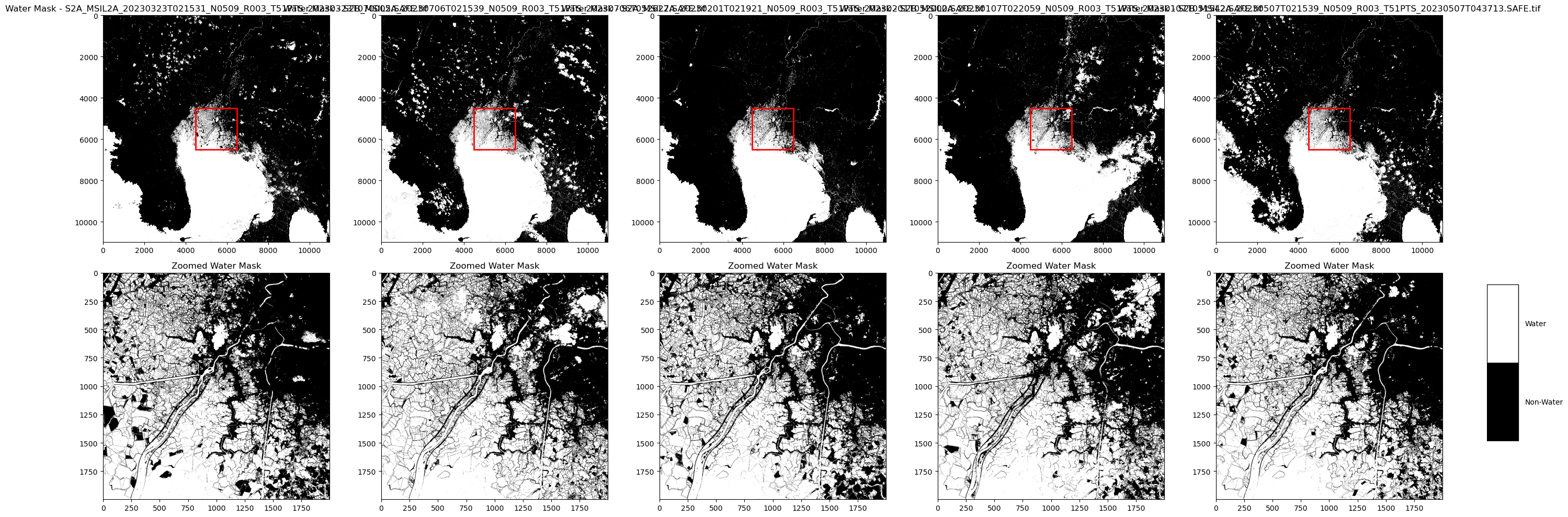
Visualization - water/no-water classification
Now try to visualize, water and -no-water areas using white and black, respectively.
- Directory Setup
Scans the output directory for .tif files and collects them for processing.
- Figure and Subplot Configuration
Creates a subplot grid with two rows for each .tif file—one for the full water mask, another for a zoomed view.
- Water Mask Creation
For each image, generates a binary water mask (1 for water, 0 for non-water) based on pixel values.
- Full Image Display
Plots the full water mask for each image in the top row using a grayscale colormap.
- Zoomed Image Display
Extracts and displays a 2000x2000 pixel zoomed area from the image center in the bottom row.
- Zoom Area Highlighting
Adds a red rectangle on the full image to indicate the zoomed section.
- Custom Legend Creation
Adds a color-coded legend to the plot with black for non-water and white for water, including labels and black borders.
- Legend Formatting
Configures the legend with a gray background, custom limits, and border visibility.
- Layout Adjustment
Ensures proper spacing and alignment of subplots and the legend.
# Directory to search for .tif files
search_directory = "output"

# Collect all .tif files in the specified directory
tif_files = [os.path.join(search_directory, f) for f in os.listdir(search_directory) if f.endswith('.tif')]

# Set up a row of subplots for each image (one for full mask, one for zoomed view)
num_files = len(tif_files)
fig, axes = plt.subplots(2, num_files, figsize=(6 * num_files, 10))

# Define colors for the water mask legend
colors = ['black', 'white']
labels = ['Non-Water', 'Water']

# Plot each .tif file in separate subplots
for idx, tif_file in enumerate(tif_files):
    with rasterio.open(tif_file) as img:
        # Calculate center coordinates
        center_x, center_y = img.width // 2, img.height // 2

        # Define the bounds for a 2,000 x 2,000 pixel window around the center
        window_size = 1000
        window = ((center_y - window_size, center_y + window_size),
                  (center_x - window_size, center_x + window_size))

        # Read the image data
        img_data = img.read(1)

        # Create a 1/0 mask for water detection (1 for water, 0 for non-water)
        water_mask = np.where(img_data > 0, 1, 0)

        # Plot the full water mask in the top row
        ax_full = axes[0, idx] if num_files > 1 else axes[0]
        show(water_mask, ax=ax_full, cmap='gray', vmin=0, vmax=1)
        ax_full.set_title(f"Water Mask - {os.path.basename(tif_file)}")

        # Set axis limits to ensure the image is fully displayed
        ax_full.set_xlim(0, img.width)
        ax_full.set_ylim(img.height, 0)

        # Draw a rectangle to highlight the zoomed area in pixel coordinates
        rect = patches.Rectangle((center_x - window_size, center_y - window_size),
                                 2000, 2000,
                                 linewidth=2, edgecolor='red', facecolor='none')

        ax_full.add_patch(rect)

        # Plot the zoomed 2,000 x 2,000 area in the bottom row
        img_array = water_mask[window[0][0]:window[0][1], window[1][0]:window[1][1]]

        ax_zoom = axes[1, idx] if num_files > 1 else axes[1]
        show(img_array, ax=ax_zoom, cmap='gray', vmin=0, vmax=1)
        ax_zoom.set_title("Zoomed Water Mask")

# Create a custom legend with black and white squares
legend_ax = fig.add_axes([0.91, 0.15, 0.03, 0.3])
legend_ax.set_facecolor('lightgray')

# Adding colored squares to the legend with a border
for i, color in enumerate(colors):
    legend_rect = patches.Rectangle((0, i), 1, 1, facecolor=color, edgecolor='black')
    legend_ax.add_patch(legend_rect)
    legend_ax.text(1.2, i + 0.5, labels[i], verticalalignment='center', color='black')

# Set the limits and hide the axes
legend_ax.set_xlim(0, 1.5)
legend_ax.set_ylim(0, len(labels))
legend_ax.axis('off')

# Create borders for the legend
for spine in legend_ax.spines.values():
    spine.set_visible(True)
    spine.set_color('black')
    spine.set_linewidth(1)

plt.tight_layout(rect=[0, 0, 0.9, 1])
plt.show()
/tmp/ipykernel_1481986/546162679.py:76: UserWarning: This figure includes Axes that are not compatible with tight_layout, so results might be incorrect.
  plt.tight_layout(rect=[0, 0, 0.9, 1])  # Adjust layout to make room for legend
Summary
This notebook processes images to create both NDWI and binary water masks, showing the full image and a zoomed-in view of each image’s center.
What To Do Next
To learn more about processing different types of satellite data, check the following articles: