Urban heat island monitoring using Sentinel-3 data in JupyterLab on CopPhil
The following example aims to present how to interact with the catalogue, download EO data products and do some basic visualization regarding land surface temperature. It is divided into four main parts:
Search for Sentinel-3 Level 2 products (SL_2_LST___) using specific filters
Download data
Cre ate a map of land surface temperature over Cebu City and the surrounding area
Calculate mean land surface temperature for specific barangays
To carry out zonal statistics it is required to provide (by user) vector files which contains eg. administrative borders. In purposes of this article, barangays borders have been used (cities.gpkg).
The SL_2_LST___ product from Sentinel-3 is used to analyze land surface temperature (LST), which is crucial for studying phenomena like the urban heat island effect. By processing this data, we can identify regions with significant temperature differences, helping to understand how urban areas experience higher temperatures compared to surrounding environments.
Prerequisites
No. 1 Access to CopPhil site
You need a CopPhil hosting account, available at https://infra.copphil.philsa.gov.ph.
No. 2 Access to JupyterLab
JupyterLab used in this article is available here: https://jupyter.infra.copphil.philsa.gov.ph/hub/login?next=%2Fhub%2F.
No. 3 Working knowledge of JupyterLab
See article Introduction to JupyterLab on CopPhil
No. 4 Using API
This is an introductory example of obtaining EODATA using API calls, in Python:
Download satellite data using API on CopPhil
No. 5 Information on Sentinel-3 mission
Page Sentinel-3 mission shows basic information on Sentinel-5P mission, which is used in this article as a source of information.
What We Are Going To Cover
Preparing your environment
Searching for the Sentinel-3 L2A products
Downloading data
Authentication
Selecting product to be downloaded
Unpack data
Download verification
Visualization
Land Surface Temperature - full image
LST over Cebu City area
Zonal statistics for barangays
LST Difference from mean around Cebu City
Zonal statistics for Temperature Difference from Mean around Cebu City
Find barangays which are the most threaten by urban heat island
Summary
Prepare your environment
Upload necessary python libraries.
# HTTP requests
import requests

# JSON parser
import json

# XML parser
import xml.etree.ElementTree as ET

# data manipulation
import numpy as np
import pandas as pd
import xarray as xr
import geopandas as gpd

# file manipulation
import zipfile
import os

# image manipulation
import matplotlib.pyplot as plt
from matplotlib import cm
from matplotlib.colors import Normalize
from matplotlib.colorbar import ColorbarBase
import matplotlib.pyplot as plt
import matplotlib.patches as mpatches
Search for the Sentinel-3 L2A products
Let’s start with obtaining some data. This part is also covered by Prerequisites No. 4.
Build a query
In order to find desired products it is needed to determinate some specific filters:
- collection_name
Sentinel-3
- product_type
SL_2_LST___
- aoi
extent (coordinates) of the area of interest (WGS84)
- search_period_start
time range - start date
- search_period_end
time range - end date
- max_cloud_cover
maximum cloud cover (%) fo the image
# base URL of the product catalogue
catalogue_odata_url = "https://catalogue.infra.copphil.philsa.gov.ph/odata/v1"

# search parameters
collection_name = "SENTINEL-3"
product_type = "SL_2_LST___"
aoi = "POLYGON((123.719867 10.440996, 124.125352 10.434967, 124.060544 10.077327, 123.725121 10.038523, 123.719867 10.440996))"
search_period_start = "2023-09-26T00:00:00.000Z"
search_period_end = "2023-09-27T00:00:00.000Z"
max_cloud_cover = 10

search_query = f"{catalogue_odata_url}/Products?$filter=Collection/Name eq '{collection_name}' and Attributes/OData.CSC.StringAttribute/any(att:att/Name eq 'productType' and att/OData.CSC.StringAttribute/Value eq '{product_type}') and OData.CSC.Intersects(area=geography'SRID=4326;{aoi}') and ContentDate/Start gt {search_period_start} and ContentDate/Start lt {search_period_end} and Attributes/OData.CSC.DoubleAttribute/any(att:att/Name eq 'cloudCover' and att/OData.CSC.DoubleAttribute/Value le {max_cloud_cover})&$expand=Attributes&$expand=Assets&$orderby=ContentDate/Start asc&$top=20"

# Print the final query
print(f"\n{search_query.replace(' ', '%20')}\n")
https://catalogue.infra.copphil.philsa.gov.ph/odata/v1/Products?$filter=Collection/Name%20eq%20'SENTINEL-3'%20and%20Attributes/OData.CSC.StringAttribute/any(att:att/Name%20eq%20'productType'%20and%20att/OData.CSC.StringAttribute/Value%20eq%20'SL_2_LST___')%20and%20OData.CSC.Intersects(area=geography'SRID=4326;POLYGON((123.719867%2010.440996,%20124.125352%2010.434967,%20124.060544%2010.077327,%20123.725121%2010.038523,%20123.719867%2010.440996))')%20and%20ContentDate/Start%20gt%202023-09-26T00:00:00.000Z%20and%20ContentDate/Start%20lt%202023-09-27T00:00:00.000Z%20and%20Attributes/OData.CSC.DoubleAttribute/any(att:att/Name%20eq%20'cloudCover'%20and%20att/OData.CSC.DoubleAttribute/Value%20le%2010)&$expand=Attributes&$expand=Assets&$orderby=ContentDate/Start%20asc&$top=20
Inspect results of the request
Show the number of found products which fits into filters requirements and get a list of names and id’s of images which fits the query.
response = requests.get(search_query).json()
result = pd.DataFrame.from_dict(response["value"])

id_list = []
for element in response['value']:
    id_value = element['Id']
    id_list.append(id_value)

for id in id_list:
    print(id)

name_list = []
for element in response['value']:
    name_value = element['Name']
    name_list.append(name_value)

for name in name_list:
    print(name)

print(f'Number of products which meets query filters: {len(result)}')
0109b9f2-826a-47c5-a257-642ccfbb3043
57dc5ac0-ee98-4224-81a4-7082a4423095
e4053e4f-6278-42e6-929b-35dc5447a05c
62fcdb5a-f8bf-4b99-ae18-9a0e7e866390
S3B_SL_2_LST____20230926T015151_20230926T015451_20230927T003232_0179_084_231_2700_PS2_O_NT_004.SEN3
S3B_SL_2_LST____20230926T015151_20230926T015451_20230926T034824_0179_084_231_2700_PS2_O_NR_004.SEN3
S3A_SL_2_LST____20230926T133243_20230926T133543_20230926T143628_0179_103_381_0000_PS1_O_NR_004.SEN3
S3A_SL_2_LST____20230926T133243_20230926T133543_20230927T232749_0179_103_381_0000_PS1_O_NT_004.SEN3
Number of products which meets query filters: 4
Get a name and id of the first image which fits the query and an info when the image was generated.
id_download = response['value'][0]['Id']
name_download = response['value'][0]['Name']
print(f'id: {id_download}, name {name_download}')

image_date = response['value'][0]['ContentDate']['Start']
print(f'Image was generated on {image_date}')
id: 0109b9f2-826a-47c5-a257-642ccfbb3043, name S3B_SL_2_LST____20230926T015151_20230926T015451_20230927T003232_0179_084_231_2700_PS2_O_NT_004.SEN3
Image was generated on 2023-09-26T01:51:50.527901Z
Download data
Authentication
Log in to the portal. If status_code=200, it means you are logged successfully.
# Provide CopPhil account credentials - replace with your own data

username = 'username'
password = 'password'
auth_server_url = "https://auth.copphil.cloudferro.com/auth/realms/copphilinfra/protocol/openid-connect/token"
data = {
    "client_id": "copphil-public",
    "grant_type": "password",
    "username": username,
    "password": password,
}

response = requests.post(auth_server_url, data=data, verify=True, allow_redirects=False)
access_token = json.loads(response.text)["access_token"]
status_code = response.status_code
print(status_code)
200
Select product to be downloaded
From the list which was provided in the previous stage and based on image name and id, download the proper image.
url_download = f'https://download.infra.copphil.philsa.gov.ph/odata/v1/Products({id_download})/$value'
url_download_using_token = url_download + '?token=' + access_token

# Download the file
pulling = requests.get(url_download_using_token)
open(f"{name_download}.zip", 'wb').write(pulling.content)
57150644
Unpack data
Unzip downloaded folder.
# Unzipping the file
with zipfile.ZipFile(f'{name_download}.zip', 'r') as zip_ref:
    zip_ref.extractall(f'{name_download}')

# Check if unzipped successfully
if os.path.exists(f'{name_download}'):
    print(f"Unzipped successfully into {name_download}")
else:
    print("Unzipping failed.")
Unzipped successfully into S3B_SL_2_LST____20230926T015151_20230926T015451_20230927T003232_0179_084_231_2700_PS2_O_NT_004.SEN3
Download verification
Take a look on obtained data - netcdf file which is containing land surface temperature values.
file_path = f"{name_download}/{name_download}/LST_in.nc"
dataset = xr.open_dataset(file_path)
print(dataset)
<xarray.Dataset> Size: 20MB
Dimensions:                 (rows: 1200, columns: 1500, orphan_pixels: 187)
Dimensions without coordinates: rows, columns, orphan_pixels
Data variables:
    LST                     (rows, columns) float32 7MB ...
    LST_orphan              (rows, orphan_pixels) float32 898kB ...
    LST_uncertainty         (rows, columns) float32 7MB ...
    LST_uncertainty_orphan  (rows, orphan_pixels) float32 898kB ...
    exception               (rows, columns) int16 4MB ...
    exception_orphan        (rows, orphan_pixels) int16 449kB ...
Attributes: (12/17)
    absolute_orbit_number:  28223
    comment:
    contact:                [email protected]
    creation_time:          20230927T003232Z
    history:                  2023-09-27T00:32:32Z: PUGCoreProcessor JobOrder...
    institution:            PS2
    ...                     ...
    source:                 IPF-SL-2 06.22
    start_offset:           58467
    start_time:             2023-09-26T01:51:50.722269Z
    stop_time:              2023-09-26T01:54:50.415934Z
    title:                  SLSTR Level 2 Product, Land Surface Temperature m...
    track_offset:           998
Visualization
Let’s start with visualization of land surface temperature retrieved from Sentinel-3 images.
Land Surface Temperature - full image
In order to visualize SL_2_LST___ data, two files has to be extracted from .SEN3 folder (product folder):
- LST_in.nc
which contains LST values
- geodetic_in.nc
which contains longitudes and latitudes
Then, LST values could be converted from Kelvin to Celsius degrees.
Values will be also filtering to remove unrealistic values (eg. related to clouds)
Map will be provided with WGS84 crs.
# Define the path to the .SEN3 folder
sen3_folder_path = f'{name_download}/{name_download}'

# Specify the LST NetCDF file to open
lst_file_path = os.path.join(sen3_folder_path, 'LST_in.nc')

# Open the LST NetCDF file using xarray
ds_lst = xr.open_dataset(lst_file_path)

# Read the LST variable
lst = ds_lst['LST']

# Check the shape and range of LST
print(f"LST shape: {lst.shape}")
print(f"Raw LST min: {lst.min().values}, max: {lst.max().values}")

# Read latitude and longitude from the geodetic file
geodetic_file_path = os.path.join(sen3_folder_path, 'geodetic_in.nc')
ds_geodetic = xr.open_dataset(geodetic_file_path)

lat = ds_geodetic['latitude_in']
lon = ds_geodetic['longitude_in']

# Convert LST from Kelvin to Celsius
processed_lst = lst - 273.15

# Filter out invalid LST values
valid_mask = processed_lst > -100  # Filtering based on realistic temperature range

# Apply the mask to the processed LST, latitude, and longitude
processed_lst_valid = processed_lst.where(valid_mask)
lat_valid = lat.where(valid_mask)
lon_valid = lon.where(valid_mask)

# Plotting the full dataset as a heatmap
plt.figure(figsize=(12, 8))

# Extract values to separate variable
heatmap_data = processed_lst_valid.values

# Generate a heatmap
plt.imshow(heatmap_data, extent=[lon_valid.min().values, lon_valid.max().values,
                                 lat_valid.min().values, lat_valid.max().values],
           aspect='auto', cmap='jet', interpolation='nearest')

plt.colorbar(label='Land Surface Temperature (°C)')
plt.xlabel('Longitude')
plt.ylabel('Latitude')
plt.title('Land Surface Temperature from Sentinel-3 SLSTR over Philippines')
plt.show()
LST shape: (1200, 1500)
Raw LST min: 224.53399658203125, max: 317.7359924316406

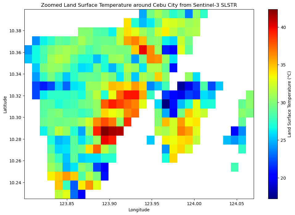
LST over Cebu City area
As the purpose of this exercise is to provide information about urban heat island phenomenon, let’s focus on some city - Cebu City and its surrounding areas.
# Define the bounding box for Cebu City
lat_min, lat_max = 10.2, 10.4
lon_min, lon_max = 123.8, 124.1

# Create a mask for the geographic bounds specific to Cebu City
geographic_mask = (lat_valid >= lat_min) & (lat_valid <= lat_max) & (lon_valid >= lon_min) & (lon_valid <= lon_max)

# Extract the valid LST, latitude, and longitude within the geographic bounds for Cebu City
final_lst_cebu = processed_lst_valid.where(geographic_mask, drop=True)
final_lat_cebu = lat_valid.where(geographic_mask, drop=True)
final_lon_cebu = lon_valid.where(geographic_mask, drop=True)

# Plotting the zoomed dataset as a heatmap for Cebu City
plt.figure(figsize=(12, 8))

# Extract values to separate variable
heatmap_data_cebu = final_lst_cebu.values

# Generate a heatmap for Cebu City
plt.imshow(heatmap_data_cebu, extent=[final_lon_cebu.min().values, final_lon_cebu.max().values,
                                      final_lat_cebu.min().values, final_lat_cebu.max().values],
           aspect='auto', cmap='jet', interpolation='nearest')

plt.colorbar(label='Land Surface Temperature (°C)')
plt.xlabel('Longitude')
plt.ylabel('Latitude')
plt.title('Zoomed Land Surface Temperature around Cebu City from Sentinel-3 SLSTR')
plt.show()
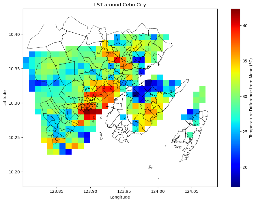
To get more geographical context, let’s add borders of barangays to the map.
# Load the city boundaries from the GeoPackage
phill_cities = gpd.read_file("cities.gpkg")


plt.figure(figsize=(12, 8))

# Plot the LST
plt.imshow(final_lst_cebu.values, extent=[final_lon_cebu.min().values, final_lon_cebu.max().values,
                                          final_lat_cebu.min().values, final_lat_cebu.max().values],
           aspect='auto', cmap='jet', interpolation='nearest')
plt.colorbar(label='Temperature Difference from Mean (°C)')
plt.xlabel('Longitude')
plt.ylabel('Latitude')
plt.title('LST around Cebu City')

# Plot the city borders in black with no fill
phill_cities.boundary.plot(ax=plt.gca(), color='black', linewidth=0.5)

# Show the final map
plt.show()
/home/ubuntu/anaconda3/envs/xcube_env/lib/python3.12/site-packages/geopandas/plotting.py:48: ShapelyDeprecationWarning: The 'type' attribute is deprecated, and will be removed in the future. You can use the 'geom_type' attribute instead.
  if geom is not None and geom.type.startswith(prefix) and not geom.is_empty:
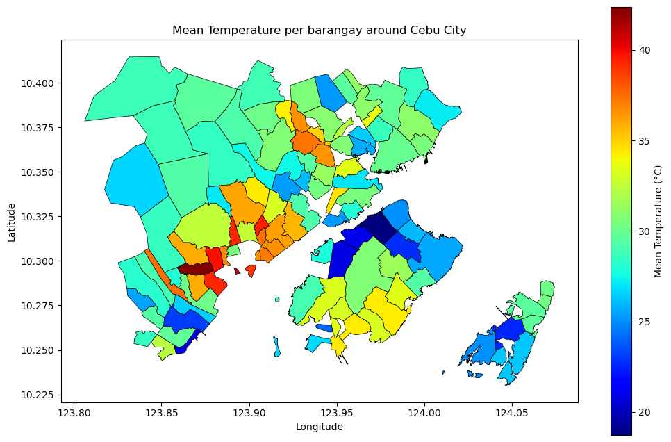
Zonal statistics for barangays
To allow us to observe regional temperature variations, let’s calculate the average LST across various cities in the Philippines, focusing on the region around Cebu City. The result is visualized on a map, where each city is color-coded based on its average temperature.
# Load the city boundaries from the GeoPackage
phill_cities = gpd.read_file("cities.gpkg")

# Convert temperature data to a GeoDataFrame for spatial join
LST_gdf = gpd.GeoDataFrame(
    {
        'LST_values': final_lst_cebu.values.flatten(),
        'geometry': gpd.points_from_xy(final_lon_cebu.values.flatten(), final_lat_cebu.values.flatten())
    },
    crs="EPSG:4326"
)

# Spatial join to map points to polygons, then group by each polygon
temp_in_polygons = gpd.sjoin(LST_gdf, phill_cities, how="inner", op='within')
mean_temp_by_city = temp_in_polygons.groupby("index_right")['LST_values'].mean()

# Add the mean temperature difference to the city GeoDataFrame for visualization
phill_cities["LST_gdf"] = phill_cities.index.map(mean_temp_by_city)

# Plot the map with cities colored by mean temperature difference
fig, ax = plt.subplots(1, 1, figsize=(12, 8))

# Normalize the color map for correct color range
norm = Normalize(vmin=phill_cities["LST_gdf"].min(), vmax=phill_cities["LST_gdf"].max())
cmap = cm.get_cmap('jet')

# Plot the city polygons with color mapped to mean temperature difference
phill_cities.plot(column='LST_gdf', cmap='jet', edgecolor='black', linewidth=0.5, ax=ax, legend=False)

# Create colorbar separately
sm = cm.ScalarMappable(cmap=cmap, norm=norm)
sm.set_array([])
fig.colorbar(sm, ax=ax, label='Mean Temperature (°C)')

# Labels and title
plt.xlabel('Longitude')
plt.ylabel('Latitude')
plt.title('Mean Temperature per barangay around Cebu City')
plt.show()
/tmp/ipykernel_3344851/538432834.py:25: MatplotlibDeprecationWarning: The get_cmap function was deprecated in Matplotlib 3.7 and will be removed in 3.11. Usematplotlib.colormaps[name]ormatplotlib.colormaps.get_cmap()orpyplot.get_cmap()instead. cmap = cm.get_cmap('jet') /home/ubuntu/anaconda3/envs/xcube_env/lib/python3.12/site-packages/geopandas/plotting.py:48: ShapelyDeprecationWarning: The 'type' attribute is deprecated, and will be removed in the future. You can use the 'geom_type' attribute instead. if geom is not None and geom.type.startswith(prefix) and not geom.is_empty:
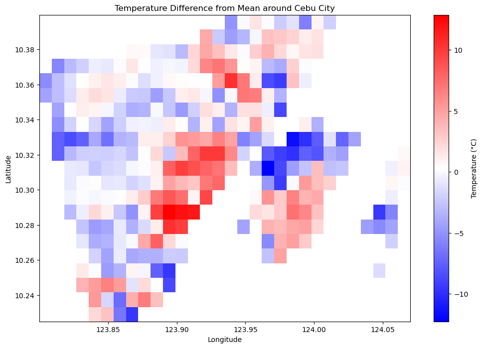
LST Difference from mean around Cebu City
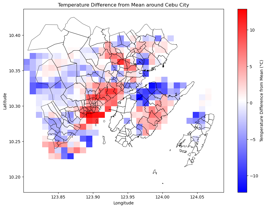
To get more context and possibility to compare LST around area, calculate the LST difference from the average temperature in the Cebu City region. The result weill be visualized on a heatmap, where areas with temperatures higher or lower than the average are shown in different colors, providing a clear view of regional temperature variations around Cebu City.
# Calculate the mean temperature within Cebu City's bounding box
mean_temp_cebu = final_lst_cebu.mean().values

# Calculate the difference between actual temperature and mean temperature
temp_diff_cebu = final_lst_cebu - mean_temp_cebu

# Plot the difference map
plt.figure(figsize=(12, 8))

# Generate a heatmap for the difference map
plt.imshow(temp_diff_cebu.values, extent=[final_lon_cebu.min().values, final_lon_cebu.max().values,
                                          final_lat_cebu.min().values, final_lat_cebu.max().values],
           aspect='auto', cmap='bwr', interpolation='nearest')

plt.colorbar(label='Temperature (°C)')
plt.xlabel('Longitude')
plt.ylabel('Latitude')
plt.title('Temperature Difference from Mean around Cebu City')
plt.show()
Again, add barangays borders to the map.
# Load the city boundaries from the GeoPackage
phill_cities = gpd.read_file("cities.gpkg")

# Step 1: Plot the temperature difference map as before
plt.figure(figsize=(12, 8))

# Plot the temperature difference heatmap
plt.imshow(temp_diff_cebu.values, extent=[final_lon_cebu.min().values, final_lon_cebu.max().values,
                                          final_lat_cebu.min().values, final_lat_cebu.max().values],
           aspect='auto', cmap='bwr', interpolation='nearest')
plt.colorbar(label='Temperature Difference from Mean (°C)')
plt.xlabel('Longitude')
plt.ylabel('Latitude')
plt.title('Temperature Difference from Mean around Cebu City')

# Plot the city borders in black with no fill
phill_cities.boundary.plot(ax=plt.gca(), color='black', linewidth=0.5)

# Show the final map
plt.show()
/home/ubuntu/anaconda3/envs/xcube_env/lib/python3.12/site-packages/geopandas/plotting.py:48: ShapelyDeprecationWarning: The 'type' attribute is deprecated, and will be removed in the future. You can use the 'geom_type' attribute instead.
  if geom is not None and geom.type.startswith(prefix) and not geom.is_empty:
Zonal statistics for Temperature Difference from Mean around Cebu City
Categorize regions based on their mean temperature difference from the average temperature around Cebu City into three categories: low (≤ 0°C), medium (1°C to 5°C), and high (> 5°C). Each category weill be assigned a specific color: blue for low, orange for medium, and red for high. The plot visualizes these categories by coloring the regions accordingly and provides a custom legend to explain the color mapping. This helps in understanding how different regions are affected by temperature variations.
temp_diff_cebu = final_lst_cebu - mean_temp_cebu  # or temp_diff_cebu = final_lst_cebu - final_lst_cebu.mean()

# Convert temp_diff_cebu to GeoDataFrame for spatial join
temp_diff_gdf = gpd.GeoDataFrame(
    {
        'temp_diff_cebu': temp_diff_cebu.values.flatten(),
        'geometry': gpd.points_from_xy(final_lon_cebu.values.flatten(), final_lat_cebu.values.flatten())
    },
    crs="EPSG:4326"
)

# Spatial join to map temperature difference to city polygons
temp_in_polygons = gpd.sjoin(temp_diff_gdf, phill_cities, how="inner", op='within')

# Calculate the mean temperature difference by city/region
mean_temp_by_city = temp_in_polygons.groupby("index_right")['temp_diff_cebu'].mean()

# Add the mean temperature difference to the city GeoDataFrame for visualization
phill_cities["mean_temp_diff"] = phill_cities.index.map(mean_temp_by_city)

# Create a categorical column based on temperature difference thresholds
conditions = [
    (phill_cities["mean_temp_diff"] <= 0),
    (phill_cities["mean_temp_diff"] > 0) & (phill_cities["mean_temp_diff"] <= 5),
    (phill_cities["mean_temp_diff"] > 5)
]
choices = ["low", "medium", "high"]
phill_cities["temp_category"] = np.select(conditions, choices, default="low")

# Define a color map as a dictionary
color_map = {
    "low": "blue",     # <= 0°C
    "medium": "orange", # 1°C to 5°C
    "high": "red"      # > 5°C
}

# Plot each category separately with specified colors
fig, ax = plt.subplots(1, 1, figsize=(12, 8))

for category, color in color_map.items():
    phill_cities[phill_cities["temp_category"] == category].plot(
        ax=ax,
        color=color,
        edgecolor="black",
        linewidth=0.5,
        label=category
    )

# Create a custom legend
legend_labels = {
    "low": "≤ 0°C",
    "medium": "1°C - 5°C",
    "high": "> 5°C"
}
patches = [mpatches.Patch(color=color_map[key], label=legend_labels[key]) for key in color_map]
plt.legend(handles=patches, title="Temperature Difference from Mean", loc="upper right")

# Labels and title
plt.xlabel('Longitude')
plt.ylabel('Latitude')
plt.title('Temperature Difference from Mean around Cebu City')
plt.show()
/home/ubuntu/anaconda3/envs/xcube_env/lib/python3.12/site-packages/geopandas/plotting.py:48: ShapelyDeprecationWarning: The 'type' attribute is deprecated, and will be removed in the future. You can use the 'geom_type' attribute instead.
  if geom is not None and geom.type.startswith(prefix) and not geom.is_empty:
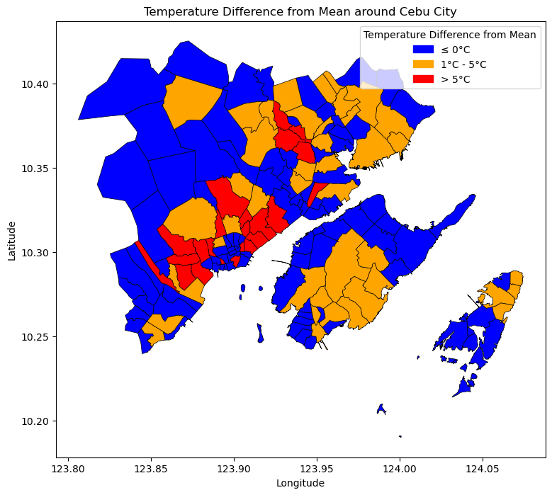
Find barangays which are the most threaten by urban heat island
Regions where the mean temperature difference exceeds 10°C.
# Filter cities/regions with a mean temperature difference greater than 10°C
above_10_diff = phill_cities[phill_cities["mean_temp_diff"] > 10]

# Display the list of region names in the 'adm4_en' column that meet the condition
adm4_above_10 = above_10_diff['adm4_en'].tolist()

print("List of regions where the mean temperature difference is above 10°C:")
for region in adm4_above_10:
    print(region)
List of regions where the mean temperature difference is above 10°C:
Labangon
Luz
Pahina San Nicolas
Punta Princesa
Regions where the mean temperature difference exceeds 5°C.
# Filter cities/regions with a mean temperature difference greater than 5°C
above_5_diff = phill_cities[phill_cities["mean_temp_diff"] > 5]

# Display the list of region names in the 'adm4_en' column that meet the condition
adm4_above_5 = above_5_diff['adm4_en'].tolist()

print("List of regions where the mean temperature difference is above 5°C:")
for region in adm4_above_5:
    print(region)
List of regions where the mean temperature difference is above 5°C:
Basak San Nicolas
Calamba
Capitol Site
Carreta
Central
Hippodromo
Kinasang-an Pardo
Labangon
Lahug
Luz
Mabolo
Mambaling
Pahina San Nicolas
Punta Princesa
T. Padilla
Tejero
Tisa
Alang-alang
Canduman
Cubacub
Pagsabungan
Subangdaku
Tawason
Summary
This notebook analyzes LST values and variations around Cebu City by processing Sentinel-3 LST data, calculating the mean temperature difference for various regions, and visualizing these differences using heatmaps. It further categorizes the regions based on temperature differences and identifies those with the highest variations, providing insights into areas with notable temperature fluctuations.
What To Do Next
To learn more about processing different types of satellite data, check the following articles: