Time series analysis of nitrogen dioxide pollution in Manila using Sentinel-5P data in JupyterLab on CopPhil
This notebook demonstrates how to obtain multiple files using the S3 protocol and perform simple time series analysis. It is divided into four main parts:
Retrieve NO₂ Tropospheric Column Number Density (NO₂ TVCD) data from Sentinel-5P.
Create a set of maps showing the average monthly NO₂ pollution over Manila.
Generate a chart illustrating the variability of NO₂ pollution over Manila from January 2022 to December 2023.
Generate a chart comparing the monthly average NO₂ pollution over Manila in 2022 and 2023.
Prerequisites
No. 1 Access to CopPhil site
You need a CopPhil hosting account, available at https://infra.copphil.philsa.gov.ph.
No. 2 Access to JupyterLab
JupyterLab used in this article is available here: https://jupyter.infra.copphil.philsa.gov.ph/hub/login?next=%2Fhub%2F.
No. 3 Working knowledge of JupyterLab
See article Introduction to JupyterLab on CopPhil
No. 4 Using API
This is an introductory example of obtaining EODATA using API calls, in Python:
Download satellite data using API on CopPhil
No. 5 Information on Sentinel-5P mission
Page Sentinel-5P mission shows basic information on Sentinel-5P mission, which is used in this article as a source of information.
No. 6 Have credentials to access EODATA ready
To obtain the necessary credentials to access EODATA, follow this article:
How to get credentials to access EODATA on CopPhil
You can generate up to 200 different keys per account.
Prepare your environment
Upload necessary python libraries.
# HTTP requests
import requests

# JSON parser
import json

# data manipulation
import pandas as pd
import numpy as np
import xarray as xr
import harp

# image manipulation
import matplotlib.pyplot as plt
import matplotlib.cm as cm
import geopandas as gpd
from collections import defaultdict

# HTTP requests
import requests

# File manipulation
import os

# Interact with s3
import boto3

# Data formats
from datetime import datetime
Connect with s3 storage - eodata
To access eodata, you must have a pair of credentials: access key and secret key. They are required to communicate with and use eodata storage. Use Prerequisite No. 7 to obtain these keys and enter them as values for variables access_key and secret_key, respectively.
If connection is successful, message Connection to bucket eodata successful. Objects found. will be printed.
access_key = ''
secret_key = ''
host = 'eodata.infra.copphil.philsa.gov.ph'

# Initialize S3 resource
s3 = boto3.resource(
    's3',
    aws_access_key_id=access_key,
    aws_secret_access_key=secret_key,
    endpoint_url=host,
)

# Verify connection by accessing the 'eodata' bucket
bucket_name = 'eodata'
try:
    bucket = s3.Bucket(bucket_name)
    # Check if the bucket is accessible by listing its contents
    objects = list(bucket.objects.limit(1))  # Limit to 1 object for testing
    if objects:
        print(f"Connection to bucket '{bucket_name}' successful. Objects found.")
    else:
        print(f"Connection to bucket '{bucket_name}' successful, but no objects found.")
except Exception as e:
    print(f"Connection to bucket '{bucket_name}' failed:", e)
Connection to bucket 'eodata' successful. Objects found.
Search for Sentinel-5P products
Let’s start with obtaining some data. Here, we are following the concept and procedures from Prerequisite No. 4. It goes without saying, however, that in this article we are going to use another set of data.
Build a query
In order to find the desired products, it is needed to determine the following filters:
- collection_name
Sentinel-5P - product_type: L2_NO2__ (tropospheric vertical NO2 column)
- processing_mode
NRTI (Near Real Time)
- aoi
extent (coordinates) of the area of interest (WGS84)
- search_period_start
time range - start date
- search_period_end
time range - end date
# Base URL of the product catalogue
catalogue_odata_url = "https://catalogue.infra.copphil.philsa.gov.ph/odata/v1"

# Search parameters
collection_name = "SENTINEL-5P"
product_type = "L2__NO2___"
processing_mode = "NRTI"
aoi = "POLYGON((120.962986 14.598416, 120.995964 14.599182, 120.999658 14.563436, 120.960348 14.567522, 120.962986 14.598416))"
search_period_start = "2022-01-01T00:00:00.000Z"
search_period_end = "2024-01-01T00:00:00.000Z"

# Construct the OData query
search_query = f"{catalogue_odata_url}/Products?$filter=Collection/Name eq '{collection_name}' and Attributes/OData.CSC.StringAttribute/any(att:att/Name eq 'productType' and att/OData.CSC.StringAttribute/Value eq '{product_type}') and Attributes/OData.CSC.StringAttribute/any(att:att/Name eq 'processingMode' and att/OData.CSC.StringAttribute/Value eq '{processing_mode}') and OData.CSC.Intersects(area=geography'SRID=4326;{aoi}') and ContentDate/Start gt {search_period_start} and ContentDate/Start lt {search_period_end}&$top=1000"

# Print the formatted URL
print(search_query)
https://catalogue.infra.copphil.philsa.gov.ph/odata/v1/Products?$filter=Collection/Name eq 'SENTINEL-5P' and Attributes/OData.CSC.StringAttribute/any(att:att/Name eq 'productType' and att/OData.CSC.StringAttribute/Value eq 'L2__NO2___') and Attributes/OData.CSC.StringAttribute/any(att:att/Name eq 'processingMode' and att/OData.CSC.StringAttribute/Value eq 'NRTI') and OData.CSC.Intersects(area=geography'SRID=4326;POLYGON((120.962986 14.598416, 120.995964 14.599182, 120.999658 14.563436, 120.960348 14.567522, 120.962986 14.598416))') and ContentDate/Start gt 2022-01-01T00:00:00.000Z and ContentDate/Start lt 2024-01-01T00:00:00.000Z&$top=1000
Inspect results of the request
Show the number of found products which fits into filters requirements and get a list of names and id’s of images which fits the query.
response = requests.get(search_query).json()
result = pd.DataFrame.from_dict(response["value"])

id_list = []
for element in response['value']:
    id_value = element['Id']
    id_list.append(id_value)


name_list = []
for element in response['value']:
    name_value = element['Name']
    name_list.append(name_value)


print(f'Number of products which meets query filters: {len(result)}')
Number of products which meets query filters: 752
Create list of paths
Parse JSON data, extracts S3Path and Name values, and combines them into a list of strings formatted as name/path. It uses list comprehensions with zip to pair paths and names efficiently and then prints the merged results.
products = json.loads(requests.get(search_query).text)

path_list = []
for item in products['value']:
    path_list.append(item['S3Path'])

name_list = []
for item in products['value']:
    name_list.append(item['Name'])


separator = '/'
result_list = [name + separator + path for name,   #create a list of merged paths and names for each image
               path in zip(path_list, name_list)]

for path in result_list[:10]:
    print(path)
/eodata/Sentinel-5P/TROPOMI/L2__NO2___/2023/11/12/S5P_NRTI_L2__NO2____20231112T060048_20231112T060548_31508_03_020500_20231112T064744/S5P_NRTI_L2__NO2____20231112T060048_20231112T060548_31508_03_020500_20231112T064744.nc
/eodata/Sentinel-5P/TROPOMI/L2__NO2___/2023/10/28/S5P_NRTI_L2__NO2____20231028T054208_20231028T054708_31295_03_020500_20231028T062948/S5P_NRTI_L2__NO2____20231028T054208_20231028T054708_31295_03_020500_20231028T062948.nc
/eodata/Sentinel-5P/TROPOMI/L2__NO2___/2023/10/30/S5P_NRTI_L2__NO2____20231030T050208_20231030T050708_31323_03_020500_20231030T054849/S5P_NRTI_L2__NO2____20231030T050208_20231030T050708_31323_03_020500_20231030T054849.nc
/eodata/Sentinel-5P/TROPOMI/L2__NO2___/2023/11/03/S5P_NRTI_L2__NO2____20231103T052708_20231103T053208_31380_03_020500_20231103T061336/S5P_NRTI_L2__NO2____20231103T052708_20231103T053208_31380_03_020500_20231103T061336.nc
/eodata/Sentinel-5P/TROPOMI/L2__NO2___/2023/11/04/S5P_NRTI_L2__NO2____20231104T050708_20231104T051208_31394_03_020500_20231104T055411/S5P_NRTI_L2__NO2____20231104T050708_20231104T051208_31394_03_020500_20231104T055411.nc
/eodata/Sentinel-5P/TROPOMI/L2__NO2___/2023/11/13/S5P_NRTI_L2__NO2____20231113T054048_20231113T054548_31522_03_020500_20231113T062651/S5P_NRTI_L2__NO2____20231113T054048_20231113T054548_31522_03_020500_20231113T062651.nc
/eodata/Sentinel-5P/TROPOMI/L2__NO2___/2023/11/16/S5P_NRTI_L2__NO2____20231116T044548_20231116T045048_31564_03_020500_20231116T053309/S5P_NRTI_L2__NO2____20231116T044548_20231116T045048_31564_03_020500_20231116T053309.nc
/eodata/Sentinel-5P/TROPOMI/L2__NO2___/2023/11/19/S5P_NRTI_L2__NO2____20231119T052548_20231119T053048_31607_03_020500_20231119T061327/S5P_NRTI_L2__NO2____20231119T052548_20231119T053048_31607_03_020500_20231119T061327.nc
/eodata/Sentinel-5P/TROPOMI/L2__NO2___/2023/11/05/S5P_NRTI_L2__NO2____20231105T045208_20231105T045708_31408_03_020500_20231105T053842/S5P_NRTI_L2__NO2____20231105T045208_20231105T045708_31408_03_020500_20231105T053842.nc
/eodata/Sentinel-5P/TROPOMI/L2__NO2___/2023/11/07/S5P_NRTI_L2__NO2____20231107T055208_20231107T055708_31437_03_020500_20231107T063850/S5P_NRTI_L2__NO2____20231107T055208_20231107T055708_31437_03_020500_20231107T063850.nc
Verify if number of paths is the same like the number of products which met query filters.
if len(path_list) == len(result_list):
    print("Number of prodcut which were found is the same like number of paths.")
else:
    print("ERROR. Number of prodcut which were found is not the same like number of paths.")
Number of prodcut which were found is the same like number of paths.
Using HARP - Atmospheric Toolbox
The HARP (Harmonized Atmospheric Retrieval Package) is an open-source software toolkit developed for processing and analyzing atmospheric composition data. It provides tools for data ingestion, filtering, resampling, and conversion, which make it particularly useful for harmonizing data from various atmospheric sensors and satellite instruments.
- A
The number of latitude edge points, calculates as follows:
(N latitude of AoI (16.0) - S latitude of AOI (14.0) / C (0.01)) + 1
- S
The latitude offset at which to start the grid (S)
- SR
The spatial resolution expressed in degrees
- B
The number of longitude edge points, calculated as follows:
(E longitude of AoI (122) - W longitude of AOI (120) / C (0.01)) + 1
- W
The longitude offset at which to start the grid (W)
- SR
The spatial resolution expressed in degrees
N = 16.00
S = 14.00
W = 120.00
E = 122.00

SR = 0.01

A = (N-S)/SR + 1
B = (E-W)/SR + 1

operations = ";".join([
    "tropospheric_NO2_column_number_density_validity>75",             # Keep pixels wich qa_value > 0.75
    "derive(surface_wind_speed {time} [m/s])",                        # Get surafe wind speed expressed in [m/s]
    "surface_wind_speed<5",                                           # Keep pixels wich wind_spped < 5 [m/s]
    # Keep variables defined below
    "keep(latitude_bounds,longitude_bounds,datetime_start,datetime_length,tropospheric_NO2_column_number_density, surface_wind_speed)",
    "derive(datetime_start {time} [days since 2000-01-01])",          # Get start time of the acquisition
    "derive(datetime_stop {time}[days since 2000-01-01])",            # Get end time of the acquisition
    "exclude(datetime_length)",                                       # Exclude datetime lenght
    f"bin_spatial({int(A)},{int(S)},{float(SR)},{int(B)},{int(W)},{float(SR)})",                       # Define bin spatial (details below)
    "derive(tropospheric_NO2_column_number_density [Pmolec/cm2])",    # Convert the NO2 units to 10^15 molec/cm^2
    "derive(latitude {latitude})",                                    # Get latitude
    "derive(longitude {longitude})",                                  # Get longitude
    "count>0"
])
Create images of NO2 monthly averaged pollution over Manilla
Define operations for temporal averaging, create new images - average NO2 pollution over defined area in specific period and import new created images as a netcdf named “mean_no2_YEAR_MONTH.nc”.
# Function to extract year and month from file path
def extract_year_month(file_path):
    # Assuming the file path contains the date in the format YYYY/MM/DD
    parts = file_path.split("/")
    year = parts[5]
    month = parts[6]
    return year, month

# Group the files by year and month
files_by_month = defaultdict(list)
for file_path in result_list:
    year, month = extract_year_month(file_path)
    files_by_month[(year, month)].append(file_path)

# Operations
reduce_operations = ";".join([
    "squash(time, (latitude, longitude, latitude_bounds, longitude_bounds))",
    "bin()"
])

# Process each month
for (year, month), files in files_by_month.items():
    # Build the file name for the monthly output
    output_filename = f"mean_no2_{year}_{month}.nc"

    # Import the product for all files in the current month
    mean_no2 = harp.import_product(files, operations, reduce_operations=reduce_operations)

    # Export the result for the current month
    harp.export_product(mean_no2, output_filename)

    print(f"Exported: {output_filename}")
Exported: mean_no2_2023_11.nc
Exported: mean_no2_2023_10.nc
Exported: mean_no2_2023_12.nc
Exported: mean_no2_2022_01.nc
Exported: mean_no2_2022_02.nc
Exported: mean_no2_2022_03.nc
Exported: mean_no2_2022_04.nc
Exported: mean_no2_2022_05.nc
Exported: mean_no2_2022_06.nc
Exported: mean_no2_2022_07.nc
Exported: mean_no2_2022_08.nc
Exported: mean_no2_2022_09.nc
Exported: mean_no2_2022_10.nc
Exported: mean_no2_2022_11.nc
Exported: mean_no2_2022_12.nc
Exported: mean_no2_2023_01.nc
Exported: mean_no2_2023_02.nc
Exported: mean_no2_2023_04.nc
Exported: mean_no2_2023_03.nc
Exported: mean_no2_2023_05.nc
Exported: mean_no2_2023_06.nc
Exported: mean_no2_2023_07.nc
Exported: mean_no2_2023_08.nc
Exported: mean_no2_2023_09.nc
Inspect one of the new created images to check variable’s name (tropospheric_NO2_column_number_density) as well as names for coordinates (latitude, longitude).
# Load the .nc file using xarray
nc_file = 'mean_no2_2023_01.nc'
mean_no2 = xr.open_dataset(nc_file)

# Inspect the dataset
print(mean_no2)
<xarray.Dataset>
Dimensions:                                 (time: 1, latitude: 200,
                                             longitude: 200, independent_2: 2)
Coordinates:
  * latitude                                (latitude) float64 14.0 ... 16.0
  * longitude                               (longitude) float64 120.0 ... 122.0
Dimensions without coordinates: time, independent_2
Data variables:
    datetime_start                          (time) datetime64[ns] ...
    tropospheric_NO2_column_number_density  (time, latitude, longitude) float64 ...
    surface_wind_speed                      (time, latitude, longitude) float64 ...
    datetime_stop                           (time) datetime64[ns] ...
    count                                   (time) int32 ...
    weight                                  (time, latitude, longitude) float32 ...
    latitude_bounds                         (latitude, independent_2) float64 ...
    longitude_bounds                        (longitude, independent_2) float64 ...
Attributes:
    Conventions:     HARP-1.0
    datetime_start:  8036.215647106482
    datetime_stop:   8066.242318217593
    history:         2024-11-13T13:07:26Z [harp-1.20.2] harp.import_product('...
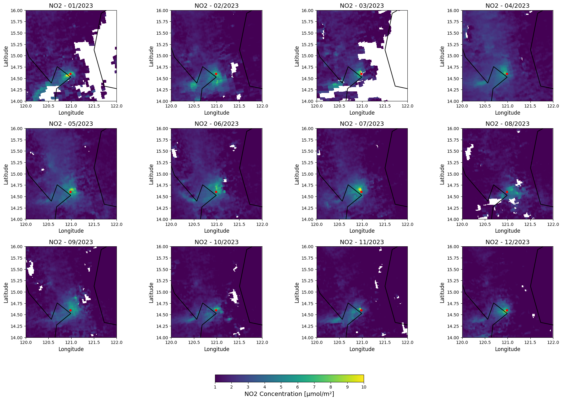
Temporal variations in NO₂ levels in Manila - set of maps
Visualize monthly mean NO₂ concentrations over the Manila region for 2023. It processes NetCDF files for each month, extracts relevant NO₂ data, and plots it on a 3x4 grid of subplots, one for each month.
It includes:
Geographic focus on Manila with boundaries and a red marker for the city.
Consistent colormap and fixed NO₂ concentration range (1–10 µmol/m²) for comparability.
Philippine borders are overlaid for geographic context, and a shared color bar enhances clarity.
The output is a detailed visualization of NO₂ variations across months. Manilla is spotted with red marker.
# List of filenames for all months (from January to December 2023)
files = [file for file in files if file.startswith('mean_no2_2023') and file.endswith('.nc')]

# Set the region boundaries for Manila
N = 16.00  # North
S = 14.00  # South
W = 120.00  # West
E = 122.00  # East

# Manila Coordinates (Lat, Lon)
manila_lat = 14.5995
manila_lon = 120.9842

# Set up the colormap and plot limits
colortable = cm.viridis
vmin, vmax = 1, 10  # Fixed color range for all plots

# Create a 3x4 grid of subplots (12 months in total)
fig, axes = plt.subplots(3, 4, figsize=(20, 15))
axes = axes.flatten()  # Flatten the 2D axes array to make indexing easier

# Load the world borders dataset for overlay (if you want it, can skip for no borders)
world = gpd.read_file(gpd.datasets.get_path('naturalearth_lowres'))
philippines = world[world.name == "Philippines"]

# Iterate through each file and plot it
for idx, file in enumerate(files):
    # Import the NO2 data for the current month
    mean_no2 = harp.import_product(file)

    # Extract the NO2 data and latitude/longitude bounds
    gridlat = mean_no2.latitude_bounds.data[:, 0]  # Southern bounds
    gridlon = mean_no2.longitude_bounds.data[:, 0]  # Western bounds
    no2 = mean_no2['tropospheric_NO2_column_number_density'].data[0, :, :]  # Use the first slice if 3D

    # Create a meshgrid for plotting
    lon_edges = np.concatenate((gridlon, [gridlon[-1] + (gridlon[1] - gridlon[0])]))
    lat_edges = np.concatenate((gridlat, [gridlat[-1] + (gridlat[1] - gridlat[0])]))

    # Remove the extra edges to match the dimensions of the NO2 data
    lon_edges = lon_edges[:-1]
    lat_edges = lat_edges[:-1]

    # Select the subplot for this month
    ax = axes[idx]

    # Plot the NO2 data
    cmesh = ax.pcolormesh(lon_edges, lat_edges, no2, shading='auto', cmap=colortable, vmin=vmin, vmax=vmax)

    # Add the borders of the Philippines
    philippines.boundary.plot(ax=ax, color='black', linewidth=1.5)

    # Plot the red point for Manila
    ax.scatter(manila_lon, manila_lat, color='red', marker='o', s=20, label='Manila')

    # Set titles and labels for each subplot
    month_name = file[14:16]  # Extract the month from the filename
    ax.set_title(f'NO2 - {month_name}/2023', fontsize=14)  # Use the month name in the title
    ax.set_xlabel('Longitude', fontsize=12)
    ax.set_ylabel('Latitude', fontsize=12)

    # Set the extent to the specified region (Manila)
    ax.set_xlim(W, E)
    ax.set_ylim(S, N)

    # Adjust aspect ratio for better visualization
    ax.set_aspect('equal')

# Adjust layout for better spacing
fig.subplots_adjust(bottom=0.1, top=0.9, left=0.05, right=0.95, hspace=0.3, wspace=0.2)

# Add a color bar below all subplots (horizontal) outside the grid
cbar = fig.colorbar(cmesh, ax=axes.ravel().tolist(), orientation='horizontal', fraction=0.02, pad=0.1)
cbar.set_label('NO2 Concentration [µmol/m²]', fontsize=14)

# Show the plot
plt.show()
/tmp/ipykernel_2737019/4263889195.py:23: FutureWarning: The geopandas.dataset module is deprecated and will be removed in GeoPandas 1.0. You can get the original 'naturalearth_lowres' data from https://www.naturalearthdata.com/downloads/110m-cultural-vectors/.
  world = gpd.read_file(gpd.datasets.get_path('naturalearth_lowres'))
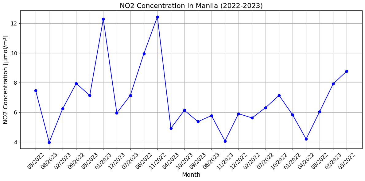
Temporal variations in NO₂ levels in Manila - charts
Visualize the monthly tropospheric NO₂ concentrations in Manila for the years 2022–2023 as a time series plot. It processes NetCDF files for each month, extracts NO₂ values closest to Manila’s geographic coordinates, and stores these in a list for visualization.
It includes:
Manila’s latitude and longitude are used to locate the nearest grid point for NO₂ data extraction.
The data is plotted against months, labeled in MM/YYYY format, showing NO₂ trends over time.
The plot includes a grid, markers for clarity, and rotated labels for better readability.
# List of filenames for all months (from January 2022 to December 2023)
files = [file for file in files if file.endswith('.nc')]

# Manila Coordinates (Lat, Lon)
manila_lat = 14.5995
manila_lon = 120.9842

# Create a list to store the NO2 values for Manila across the months
manila_no2_values = []

# Iterate through each file and extract NO2 values at Manila's coordinates
for file in files:
    # Import the NO2 data for the current month
    mean_no2 = harp.import_product(file)

    # Extract the NO2 data and latitude/longitude values
    gridlat = mean_no2.latitude.data  # Latitude values
    gridlon = mean_no2.longitude.data  # Longitude values
    no2 = mean_no2['tropospheric_NO2_column_number_density'].data[0, :, :]  # Assuming 3D: time, lat, lon

    # Find the index of the nearest latitude and longitude to Manila's coordinates
    lat_idx = (np.abs(gridlat - manila_lat)).argmin()
    lon_idx = (np.abs(gridlon - manila_lon)).argmin()

    # Extract the NO2 value for Manila
    manila_no2_value = no2[lat_idx, lon_idx]
    manila_no2_values.append(manila_no2_value)

# Create a time series plot for the NO2 values in Manila
months = [f"{file[14:16]}/{file[9:13]}" for file in files]  # Extract the month and year from the filename

plt.figure(figsize=(12, 6))
plt.plot(months, manila_no2_values, marker='o', color='b', linestyle='-', markersize=6, label='NO2 Concentration')

# Add labels and title
plt.title('NO2 Concentration in Manila (2022-2023)', fontsize=16)
plt.xlabel('Month', fontsize=14)
plt.ylabel('NO2 Concentration [µmol/m²]', fontsize=14)

# Rotate the month labels for better visibility
plt.xticks(rotation=45, fontsize=12)
plt.yticks(fontsize=12)

# Add a grid for better readability
plt.grid(True)

# Show the plot
plt.tight_layout()
plt.show()
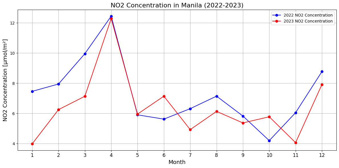
Temporal variations in NO₂ levels in Manila - year to year
Visualize monthly NO₂ concentration data for Manila across 2022–2023 and visualizes it as a time series. For each month, it extracts the NO₂ value closest to Manila’s geographic coordinates from the dataset and compiles them into a list.
It includes:
Manila’s latitude and longitude are used to locate the nearest grid point in the data.
The resulting NO₂ values are plotted against months, showing trends over time with clear markers and gridlines.
The plot uses rotated labels and formatting to enhance readability, providing a comprehensive view of NO₂ concentration variations.
# List of filenames for all months (from January 2022 to December 2023)
files_2022 = [file for file in files if file.startswith('mean_no2_2022') and file.endswith('.nc')]

files_2023 = [file for file in files if file.startswith('mean_no2_2023') and file.endswith('.nc')]


# Manila Coordinates (Lat, Lon)
manila_lat = 14.5995
manila_lon = 120.9842

# Create lists to store the NO2 values for Manila across 2022 and 2023
manila_no2_values_2022 = []
manila_no2_values_2023 = []

# Function to extract NO2 values for each year
def extract_no2_values(files, year_values_list):
    for file in files:
        # Import the NO2 data for the current month
        mean_no2 = harp.import_product(file)

        # Extract the NO2 data and latitude/longitude values
        gridlat = mean_no2.latitude.data  # Latitude values
        gridlon = mean_no2.longitude.data  # Longitude values
        no2 = mean_no2['tropospheric_NO2_column_number_density'].data[0, :, :]  # Assuming 3D: time, lat, lon

        # Find the index of the nearest latitude and longitude to Manila's coordinates
        lat_idx = (np.abs(gridlat - manila_lat)).argmin()
        lon_idx = (np.abs(gridlon - manila_lon)).argmin()

        # Extract the NO2 value for Manila
        manila_no2_value = no2[lat_idx, lon_idx]
        year_values_list.append(manila_no2_value)

# Extract NO2 values for 2022 and 2023
extract_no2_values(files_2022, manila_no2_values_2022)
extract_no2_values(files_2023, manila_no2_values_2023)

# Create a common list for months (1-12 for both years)
months = np.arange(1, 13)

# Plotting the NO2 values for Manila across 2022 and 2023
plt.figure(figsize=(12, 6))

# Plot 2022 data (first line, blue)
plt.plot(months, manila_no2_values_2022, marker='o', color='b', linestyle='-', markersize=6, label='2022 NO2 Concentration')

# Plot 2023 data (second line, red)
plt.plot(months, manila_no2_values_2023, marker='o', color='r', linestyle='-', markersize=6, label='2023 NO2 Concentration')

# Add labels and title
plt.title('NO2 Concentration in Manila (2022-2023)', fontsize=16)
plt.xlabel('Month', fontsize=14)
plt.ylabel('NO2 Concentration [µmol/m²]', fontsize=14)

# Add x-axis ticks for months (1 to 12)
plt.xticks(months, fontsize=12)

# Add a grid for better readability
plt.grid(True)

# Add a legend
plt.legend()

# Show the plot
plt.tight_layout()
plt.show()
Summary
The tutorial explained how to analyze NO₂ concentrations through the time. The first time series visualizes monthly NO₂ maps for 2023, highlighting geographic patterns. The second and third create time series for 2022–2023, showing monthly trends in NO₂ levels. Together, they provide spatial and temporal insights into air pollution.